


Set priorities and weights for data through the impact of cell image labels on model performance.
One of the major obstacles for many machine learning tasks is the lack of labeled data. Labeling data can take a long time and be expensive, so many times it is unreasonable to try to use machine learning methods to solve the problem.
In order to solve this problem, a field called active learning emerged in the field of machine learning. Active learning is a method in machine learning that provides a framework for prioritizing unlabeled data samples based on the labeled data that the model has already seen. If you want to
Segmentation and classification technologies for cell imaging are a rapidly developing field of research. Just like in other machine learning fields, data annotation is very expensive, and the quality requirements for data annotation are also very high. To address this problem, this article introduces an active learning end-to-end workflow for red blood cell and white blood cell image classification tasks.
Our goal is to combine biology and active learning and help others use active learning methods to solve similar and more complex tasks in biology.
This article mainly consists of three parts:
- Cell image preprocessing - here we will introduce how to preprocess unsegmented blood cell images.
- Use CellProfiler to extract cell features - shows how to extract morphological features from biological cell photo images to be used as features for machine learning models.
- Use active learning - shows a comparative experiment simulating the use of active learning and not using active learning.
Cell image preprocessing
We will use the blood cell image dataset licensed under MIT (GitHub and Kaggle). Each image is labeled according to red blood cell (RBC) and white blood cell (WBC) classification. There are additional tags for these four types of leukocytes (eosinophils, lymphocytes, monocytes, and neutrophils), but these were not used in this study.
Here is an example of a full-size original image from the dataset:

Create sample DF
The original dataset contains an export .py script that parses the XML annotations into a CSV table containing the filename, cell type label, and bounding box for each cell.
The original script did not include the cell_id column, but we wanted to classify individual cells, so we modified the code slightly to add that column and added a filename column that included image_id and cell_id:
import os, sys, randomimport xml.etree.ElementTree as ETfrom glob import globimport pandas as pdfrom shutil import copyfileannotations = glob('BCCD_Dataset/BCCD/Annotations/*.xml')df = []for file in annotations:#filename = file.split('/')[-1].split('.')[0] + '.jpg'#filename = str(cnt) + '.jpg'filename = file.split('\')[-1]filename =filename.split('.')[0] + '.jpg'row = []parsedXML = ET.parse(file)cell_id = 0for node in parsedXML.getroot().iter('object'):blood_cells = node.find('name').textxmin = int(node.find('bndbox/xmin').text)xmax = int(node.find('bndbox/xmax').text)ymin = int(node.find('bndbox/ymin').text)ymax = int(node.find('bndbox/ymax').text)row = [filename, cell_id, blood_cells, xmin, xmax, ymin, ymax]df.append(row)cell_id += 1data = pd.DataFrame(df, columns=['filename', 'cell_id', 'cell_type', 'xmin', 'xmax', 'ymin', 'ymax'])data['image_id'] = data['filename'].apply(lambda x: int(x[-7:-4]))data[['filename', 'image_id', 'cell_id', 'cell_type', 'xmin', 'xmax', 'ymin', 'ymax']].to_csv('bccd.csv', index=False)
Crop
To be able to process the data, the first step is to crop the full-size image based on the bounding box coordinates. This produces many images of cells of varying sizes:


The cropped code is as follows:
import osimport pandas as pdfrom PIL import Imagedef crop_cell(row):"""crop_cell(row)given a pd.Series row of the dataframe, load row['filename'] with PIL,crop it to the box row['xmin'], row['xmax'], row['ymin'], row['ymax']save the cropped image,return cropped filename"""input_dir = 'BCCDJPEGImages'output_dir = 'BCCDcropped'# open imageim = Image.open(f"{input_dir}{row['filename']}")# size of the image in pixelswidth, height = im.size# setting the points for cropped imageleft = row['xmin']bottom = row['ymax']right = row['xmax']top = row['ymin']# cropped imageim1 = im.crop((left, top, right, bottom))cropped_fname = f"BloodImage_{row['image_id']:03d}_{row['cell_id']:02d}.jpg"# shows the image in image viewer# im1.show()# save imagetry:im1.save(f"{output_dir}{cropped_fname}")except:return 'error while saving image'return cropped_fnameif __name__ == "__main__":# load labels csv into Pandas DataFramefilepath = "BCCDdataset2-masterlabels.csv"df = pd.read_csv(filepath)# iterate through cells, crop each cell, and save cropped cell to filedataset_df['cell_filename'] = dataset_df.apply(crop_cell, axis=1)
The above are all the preprocessing operations we have done. Now, we continue to use CellProfiler to extract features.
Extract cell features using CellProfiler
CellProfiler is a free and open source image analysis software that can automatically make quantitative measurements from large-scale cell images. CellProfiler also contains a GUI interface that allows us to perform visual operations
First download CellProfiler. If CellProfiler cannot be opened, you may need to install the Visual C release package. Please refer to the official website for specific installation methods.
Open the software to load the image. If you want to build a pipeline, you can find the list of available functions provided by CellProfiler on its official website. Most functions are divided into three main groups: image processing, target processing and measurement.
Commonly used functions are as follows:
Image processing - Convert to grayscale image:

Object target processing - Identify main objects

测量 - 测量对象强度

CellProfiler可以将输出为CSV文件或者保存指定数据库中。这里我们将输出保存为CSV文件,然后将其加载到Python进行进一步处理。
说明:CellProfiler还可以将你处理图像的流程保存并进行分享。
主动学习
我们现在已经有了训练需要的搜有数据,现在可以开始试验使用主动学习策略是否可以通过更少的数据标记获得更高的准确性。 我们的假设是:使用主动学习可以通过大量减少在细胞分类任务上训练机器学习模型所需的标记数据量来节省宝贵的时间和精力。
主动学习框架
在深入研究实验之前,我们希望对modAL进行快速介绍: modAL是Python的活跃学习框架。 它提供了Sklearn API,因此可以非常容易的将其集成到代码中。 该框架可以轻松地使用不同的主动学习策略。 他们的文档也很清晰,所以建议从它开始你的一个主动学习项目。
主动学习与随机学习
为了验证假设,我们将进行一项实验,将添加新标签数据的随机子抽样策略与主动学习策略进行比较。开始用一些相同的标记样本训练2个Logistic回归估计器。然后将在一个模型中使用随机策略,在第二个模型中使用主动学习策略。
我们首先为实验准备数据,加载由Cell Profiler言创建的特征。 这里过滤了无色血细胞的血小板,只保留红和白细胞(将问题简化,并减少数据量) 。所以现在我们正在尝试解决二进制分类问题 - RBC与WBC。使用Sklearn Label的label encoder进行编码,并拆分数据集进行训练和测试。
# imports for the whole experimentimport numpy as npfrom matplotlib import pyplot as pltfrom modAL import ActiveLearnerimport pandas as pdfrom modAL.uncertainty import uncertainty_samplingfrom sklearn import preprocessingfrom sklearn.metrics import , average_precision_scorefrom sklearn.linear_model import LogisticRegression# upload the cell profiler features for each celldata = pd.read_csv('Zaretski_Image_All.csv')# filter plateletsdata = data[data['cell_type'] != 'Platelets']# define the labeltarget = 'cell_type'label_encoder = preprocessing.LabelEncoder()y = label_encoder.fit_transform(data[target])# take the learning features onlyX = data.iloc[:, 5:]# create training and testing setsX_train, X_test, y_train, y_test = train_test_split(X.to_numpy(), y, test_size=0.33, random_state=42)
下一步就是创建模型
<span style="color: rgb(89, 89, 89); margin: 0px; padding: 0px; background: none 0% 0% / auto repeat scroll padding-box border-box rgba(0, 0, 0, 0);">dummy_learner</span> <span style="color: rgb(215, 58, 73); margin: 0px; padding: 0px; background: none 0% 0% / auto repeat scroll padding-box border-box rgba(0, 0, 0, 0);">=</span> <span style="color: rgb(89, 89, 89); margin: 0px; padding: 0px; background: none 0% 0% / auto repeat scroll padding-box border-box rgba(0, 0, 0, 0);">LogisticRegression</span>()<br><span style="color: rgb(89, 89, 89); margin: 0px; padding: 0px; background: none 0% 0% / auto repeat scroll padding-box border-box rgba(0, 0, 0, 0);">active_learner</span> <span style="color: rgb(215, 58, 73); margin: 0px; padding: 0px; background: none 0% 0% / auto repeat scroll padding-box border-box rgba(0, 0, 0, 0);">=</span> <span style="color: rgb(89, 89, 89); margin: 0px; padding: 0px; background: none 0% 0% / auto repeat scroll padding-box border-box rgba(0, 0, 0, 0);">ActiveLearner</span>(<br><span style="color: rgb(89, 89, 89); margin: 0px; padding: 0px; background: none 0% 0% / auto repeat scroll padding-box border-box rgba(0, 0, 0, 0);">estimator</span><span style="color: rgb(215, 58, 73); margin: 0px; padding: 0px; background: none 0% 0% / auto repeat scroll padding-box border-box rgba(0, 0, 0, 0);">=</span><span style="color: rgb(89, 89, 89); margin: 0px; padding: 0px; background: none 0% 0% / auto repeat scroll padding-box border-box rgba(0, 0, 0, 0);">LogisticRegression</span>(),<br><span style="color: rgb(89, 89, 89); margin: 0px; padding: 0px; background: none 0% 0% / auto repeat scroll padding-box border-box rgba(0, 0, 0, 0);">query_strategy</span><span style="color: rgb(215, 58, 73); margin: 0px; padding: 0px; background: none 0% 0% / auto repeat scroll padding-box border-box rgba(0, 0, 0, 0);">=</span><span style="color: rgb(89, 89, 89); margin: 0px; padding: 0px; background: none 0% 0% / auto repeat scroll padding-box border-box rgba(0, 0, 0, 0);">uncertainty_sampling</span>()<br>)
dummy_learner是使用随机策略的模型,而active_learner是使用主动学习策略的模型。为了实例化一个主动学习模型,我们使用modAL包中的ActiveLearner对象。在“estimator”字段中,可以插入任何sklearnAPI兼容的模型。在query_strategy '字段中可以选择特定的主动学习策略。这里使用“uncertainty_sampling()”。这方面更多的信息请查看modAL文档。
将训练数据分成两组。第一个是训练数据,我们知道它的标签,会用它来训练模型。第二个是验证数据,虽然标签也是已知的,但是我们假装不知道它的标签,并通过模型预测的标签和实际标签进行比较来评估模型的性能。然后我们将训练的数据样本数设置成5。
# the training size that we will start withbase_size = 5# the 'base' data that will be the training set for our modelX_train_base_dummy = X_train[:base_size]X_train_base_active = X_train[:base_size]y_train_base_dummy = y_train[:base_size]y_train_base_active = y_train[:base_size]# the 'new' data that will simulate unlabeled data that we pick a sample from and label itX_train_new_dummy = X_train[base_size:]X_train_new_active = X_train[base_size:]y_train_new_dummy = y_train[base_size:]y_train_new_active = y_train[base_size:]
我们训练298个epoch,在每个epoch中,将训练这俩个模型和选择下一个样本,并根据每个模型的策略选择是否将样本加入到我们的“基础”数据中,并在每个epoch中测试其准确性。因为分类是不平衡的,所以使用平均精度评分来衡量模型的性能。
在随机策略中选择下一个样本,只需将下一个样本添加到虚拟数据集的“新”组中,这是因为数据集已经是打乱的的,因此不需要在进行这个操作。对于主动学习,将使用名为“query”的ActiveLearner方法,该方法获取“新”组的未标记数据,并返回他建议添加到训练“基础”组的样本索引。被选择的样本都将从组中删除,因此样本只能被选择一次。
# arrays to accumulate the scores of each simulation along the epochsdummy_scores = []active_scores = []# number of desired epochsrange_epoch = 298# running the experimentfor i in range(range_epoch):# train the models on the 'base' datasetactive_learner.fit(X_train_base_active, y_train_base_active)dummy_learner.fit(X_train_base_dummy, y_train_base_dummy)# evaluate the modelsdummy_pred = dummy_learner.predict(X_test)active_pred = active_learner.predict(X_test)# accumulate the scoresdummy_scores.append(average_precision_score(dummy_pred, y_test))active_scores.append(average_precision_score(active_pred, y_test))# pick the next sample in the random strategy and randomly# add it to the 'base' dataset of the dummy learner and remove it from the 'new' datasetX_train_base_dummy = np.append(X_train_base_dummy, [X_train_new_dummy[0, :]], axis=0)y_train_base_dummy = np.concatenate([y_train_base_dummy, np.array([y_train_new_dummy[0]])], axis=0)X_train_new_dummy = X_train_new_dummy[1:]y_train_new_dummy = y_train_new_dummy[1:]# pick next sample in the active strategyquery_idx, query_sample = active_learner.query(X_train_new_active)# add the index to the 'base' dataset of the active learner and remove it from the 'new' datasetX_train_base_active = np.append(X_train_base_active, X_train_new_active[query_idx], axis=0)y_train_base_active = np.concatenate([y_train_base_active, y_train_new_active[query_idx]], axis=0)X_train_new_active = np.concatenate([X_train_new_active[:query_idx[0]], X_train_new_active[query_idx[0] + 1:]], axis=0)y_train_new_active = np.concatenate([y_train_new_active[:query_idx[0]], y_train_new_active[query_idx[0] + 1:]], axis=0)
结果如下:
plt.plot(list(range(range_epoch)), active_scores, label='Active Learning')plt.plot(list(range(range_epoch)), dummy_scores, label='Dummy')plt.xlabel('number of added samples')plt.ylabel('average precision score')plt.legend(loc='lower right')plt.savefig("models robustness vs dummy.png", bbox_inches='tight')plt.show()

策略之间的差异还是很大的,可以看到主动学习只使用25个样本就可以达到平均精度0.9得分! 而使用随机的策略则需要175个样本才能达到相同的精度!
In addition, the score of the model with active learning strategy is close to 0.99, while the score of the random model stops at around 0.95! If we use all the data, then their final scores are the same, but the purpose of our research is to train on the premise of a small amount of labeled data, so only 300 random samples in the data set are used.
Summary
This paper demonstrates the benefits of using active learning for cell imaging tasks. Active learning is a set of methods in machine learning that prioritize solutions for unlabeled data examples based on the impact their labels have on model performance. Since labeling data is a task involving many resources (money and time), it is necessary to judge which samples to label which can maximize the performance of the model.
Cell imaging has made tremendous contributions to the fields of biology, medicine and pharmacology. In the past, analyzing cell images required valuable professional human capital, but the emergence of technologies like active learning provides a very good solution for fields such as medicine that require large amounts of human-annotated data sets.
The above is the detailed content of A brief analysis of active learning of cell image data. For more information, please follow other related articles on the PHP Chinese website!

 解读CRISP-ML(Q):机器学习生命周期流程Apr 08, 2023 pm 01:21 PM
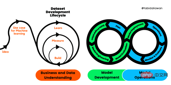
译者 | 布加迪审校 | 孙淑娟目前,没有用于构建和管理机器学习(ML)应用程序的标准实践。机器学习项目组织得不好,缺乏可重复性,而且从长远来看容易彻底失败。因此,我们需要一套流程来帮助自己在整个机器学习生命周期中保持质量、可持续性、稳健性和成本管理。图1. 机器学习开发生命周期流程使用质量保证方法开发机器学习应用程序的跨行业标准流程(CRISP-ML(Q))是CRISP-DM的升级版,以确保机器学习产品的质量。CRISP-ML(Q)有六个单独的阶段:1. 业务和数据理解2. 数据准备3. 模型
 基于因果森林算法的决策定位应用Apr 08, 2023 am 11:21 AM
译者 | 朱先忠审校 | 孙淑娟在我之前的博客中,我们已经了解了如何使用因果树来评估政策的异质处理效应。如果你还没有阅读过,我建议你在阅读本文前先读一遍,因为我们在本文中认为你已经了解了此文中的部分与本文相关的内容。为什么是异质处理效应(HTE:heterogenous treatment effects)呢?首先,对异质处理效应的估计允许我们根据它们的预期结果(疾病、公司收入、客户满意度等)选择提供处理(药物、广告、产品等)的用户(患者、用户、客户等)。换句话说,估计HTE有助于我
 2023年机器学习的十大概念和技术Apr 04, 2023 pm 12:30 PM
机器学习是一个不断发展的学科,一直在创造新的想法和技术。本文罗列了2023年机器学习的十大概念和技术。 本文罗列了2023年机器学习的十大概念和技术。2023年机器学习的十大概念和技术是一个教计算机从数据中学习的过程,无需明确的编程。机器学习是一个不断发展的学科,一直在创造新的想法和技术。为了保持领先,数据科学家应该关注其中一些网站,以跟上最新的发展。这将有助于了解机器学习中的技术如何在实践中使用,并为自己的业务或工作领域中的可能应用提供想法。2023年机器学习的十大概念和技术:1. 深度神经网
 使用PyTorch进行小样本学习的图像分类Apr 09, 2023 am 10:51 AM
近年来,基于深度学习的模型在目标检测和图像识别等任务中表现出色。像ImageNet这样具有挑战性的图像分类数据集,包含1000种不同的对象分类,现在一些模型已经超过了人类水平上。但是这些模型依赖于监督训练流程,标记训练数据的可用性对它们有重大影响,并且模型能够检测到的类别也仅限于它们接受训练的类。由于在训练过程中没有足够的标记图像用于所有类,这些模型在现实环境中可能不太有用。并且我们希望的模型能够识别它在训练期间没有见到过的类,因为几乎不可能在所有潜在对象的图像上进行训练。我们将从几个样本中学习
 LazyPredict:为你选择最佳ML模型!Apr 06, 2023 pm 08:45 PM
本文讨论使用LazyPredict来创建简单的ML模型。LazyPredict创建机器学习模型的特点是不需要大量的代码,同时在不修改参数的情况下进行多模型拟合,从而在众多模型中选出性能最佳的一个。 摘要本文讨论使用LazyPredict来创建简单的ML模型。LazyPredict创建机器学习模型的特点是不需要大量的代码,同时在不修改参数的情况下进行多模型拟合,从而在众多模型中选出性能最佳的一个。本文包括的内容如下:简介LazyPredict模块的安装在分类模型中实施LazyPredict
 Mango:基于Python环境的贝叶斯优化新方法Apr 08, 2023 pm 12:44 PM
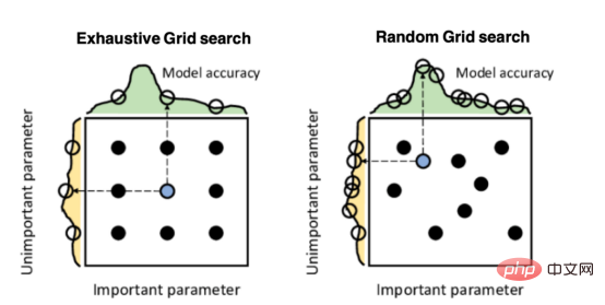
译者 | 朱先忠审校 | 孙淑娟引言模型超参数(或模型设置)的优化可能是训练机器学习算法中最重要的一步,因为它可以找到最小化模型损失函数的最佳参数。这一步对于构建不易过拟合的泛化模型也是必不可少的。优化模型超参数的最著名技术是穷举网格搜索和随机网格搜索。在第一种方法中,搜索空间被定义为跨越每个模型超参数的域的网格。通过在网格的每个点上训练模型来获得最优超参数。尽管网格搜索非常容易实现,但它在计算上变得昂贵,尤其是当要优化的变量数量很大时。另一方面,随机网格搜索是一种更快的优化方法,可以提供更好的
 人工智能自动获取知识和技能,实现自我完善的过程是什么Aug 24, 2022 am 11:57 AM
实现自我完善的过程是“机器学习”。机器学习是人工智能核心,是使计算机具有智能的根本途径;它使计算机能模拟人的学习行为,自动地通过学习来获取知识和技能,不断改善性能,实现自我完善。机器学习主要研究三方面问题:1、学习机理,人类获取知识、技能和抽象概念的天赋能力;2、学习方法,对生物学习机理进行简化的基础上,用计算的方法进行再现;3、学习系统,能够在一定程度上实现机器学习的系统。
 超参数优化比较之网格搜索、随机搜索和贝叶斯优化Apr 04, 2023 pm 12:05 PM
本文将详细介绍用来提高机器学习效果的最常见的超参数优化方法。 译者 | 朱先忠审校 | 孙淑娟简介通常,在尝试改进机器学习模型时,人们首先想到的解决方案是添加更多的训练数据。额外的数据通常是有帮助(在某些情况下除外)的,但生成高质量的数据可能非常昂贵。通过使用现有数据获得最佳模型性能,超参数优化可以节省我们的时间和资源。顾名思义,超参数优化是为机器学习模型确定最佳超参数组合以满足优化函数(即,给定研究中的数据集,最大化模型的性能)的过程。换句话说,每个模型都会提供多个有关选项的调整“按钮


Hot AI Tools

Undresser.AI Undress
AI-powered app for creating realistic nude photos

AI Clothes Remover
Online AI tool for removing clothes from photos.

Undress AI Tool
Undress images for free

Clothoff.io
AI clothes remover

AI Hentai Generator
Generate AI Hentai for free.

Hot Article
Hot Tools

Dreamweaver Mac version
Visual web development tools

VSCode Windows 64-bit Download
A free and powerful IDE editor launched by Microsoft

MinGW - Minimalist GNU for Windows
This project is in the process of being migrated to osdn.net/projects/mingw, you can continue to follow us there. MinGW: A native Windows port of the GNU Compiler Collection (GCC), freely distributable import libraries and header files for building native Windows applications; includes extensions to the MSVC runtime to support C99 functionality. All MinGW software can run on 64-bit Windows platforms.

PhpStorm Mac version
The latest (2018.2.1) professional PHP integrated development tool

SAP NetWeaver Server Adapter for Eclipse
Integrate Eclipse with SAP NetWeaver application server.

