 Technology peripherals
 AI
AI From VAE to Diffusion Model: An article explaining the new paradigm of using texts to generate diagrams
From VAE to Diffusion Model: An article explaining the new paradigm of using texts to generate diagrams
1 Foreword
Fifteen months after the release of DALL·E, OpenAI brought the sequel DALL·E 2 this spring, which quickly occupied the market with its more stunning effects and rich playability. Headlines from major AI communities. In recent years, with the emergence of Generative Adversarial Networks (GAN), Variational Autoencoders (VAE), and Diffusion models, deep learning has demonstrated its powerful image generation capabilities to the world; together with GPT-3, BERT Waiting for the success of NLP models, humans are gradually breaking the information boundaries between text and images.
In DALL·E 2, just enter a simple text (prompt), and it can generate multiple 1024*1024 high-definition images. These images can even express unconventional semantics to create imaginative visual effects in a surreal form, such as "An astronaut riding a horse in a photorealistic style" in Figure 1.
 Figure 1. DALL·E 2 generation example
This article will provide an in-depth explanation of how new paradigms such as DALL·E can create many amazing images through text. The article covers a lot of background knowledge and The introduction of basic technologies is also suitable for readers who are new to the field of image generation.
2 Image generation

Figure 2. Mainstream image generation methods
Since the birth of Generative Adversarial Network (GAN) in 2014, images Generative research has become an important frontier topic in deep learning and even the entire field of artificial intelligence. At this stage, technological development has reached the point where fakes can be confused with real ones. In addition to the well-known Generative Adversarial Network (GAN), mainstream methods also include variational autoencoders (VAE) and flow-based models (Flow-based models), as well as diffusion models (Diffusion models) that have attracted much attention recently. With the help of Figure 2, we explore the characteristics and differences of each method.
2.1 Generative Adversarial Network (GAN)
The full name of GAN is G enerative A dversarial N etworks, it is not difficult to read from the name that "Adversarial" is the essence of its success. The idea of confrontation is inspired by game theory. While training the generator (Generator), train a discriminator (Discriminator) to judge whether the input is a real image or a generated image. The two compete with each other in a minimax game and become stronger. , such as formula (1). When an image sufficient to "fool" is generated from random noise, we believe that the data distribution of the real image is well fitted, and a large number of realistic images can be generated through sampling.

GAN is the most widely used technology in generative models and shines in many data synthesis scenarios such as images, videos, speech and NLP. In addition to generating content directly from random noise, we can also add conditions (such as classification labels) as inputs to the generator and discriminator, so that the generated results conform to the attributes of the conditional input, allowing the generated content to be controlled. Although GAN has outstanding effects, due to the existence of game mechanism, its training stability is poor and prone to mode collapse. How to make the model reach the game equilibrium point smoothly is also a hot research topic in GAN.
2.2 Variational Autoencoder (VAE)
Variational Autoencoder (Variational Autoencoder) is a variant of the autoencoder. The traditional autoencoder is designed to operate in an unsupervised manner. The way to train a neural network is to compress the original input into an intermediate representation and restore it into two processes. The former converts the original high-dimensional input into a low-dimensional hidden layer encoding through the encoder (Encoder), and the latter passes through the decoder (Decoder). ) to reconstruct the data from the encoding. It is not difficult to see that the goal of the autoencoder is to learn an identity function. We can use cross-entropy (Cross-entropy) or mean square error (Mean Square Error) to construct a reconstruction loss to quantify the difference between the input and the output. As shown in Figure 3, during the above process we obtain a low-dimensional hidden layer encoding, which captures the potential attributes of the original data and can be used for data compression and feature representation.

Figure 3. Latent attribute encoding of autoencoder
Since the autoencoder only focuses on the reconstruction ability of hidden layer encoding, its hidden layer spatial distribution is often It is irregular and uneven. Random sampling or interpolation in the continuous hidden layer space to obtain a set of codes usually produces meaningless and uninterpretable generation results. In order to construct a regular hidden layer space so that we can randomly sample and smoothly interpolate different potential attributes, and finally generate meaningful images through the decoder, researchers proposed the variational autoencoder in 2014.
The variational autoencoder no longer maps the input to a fixed encoding in the hidden layer space, but converts it into a probability distribution estimate of the hidden layer space. For convenience of expression, we assume that the prior distribution is a standard Gaussian distribution. Similarly, we train a probabilistic decoder model to map from the hidden layer spatial distribution to the real data distribution. When given an input, we estimate the parameters of the distribution (the mean and covariance of the multivariate Gaussian model) through the posterior distribution, and sample from this distribution. We can use reparameterization techniques to make the sampling differentiable (as a random variable) , and finally the distribution about is output through the probability decoder, as shown in Figure 4. In order to make the generated image as realistic as possible, we need to solve for the posterior distribution, with the goal of maximizing the log-likelihood of the real image.

Figure 4. Sampling generation process of variational autoencoder
Unfortunately, the true posterior distribution according to the Bayesian model contains Integrals on continuous spaces cannot be solved directly. In order to solve the above problems, the variational autoencoder uses the variational inference method, introduces a learnable probability encoder to approximate the real posterior distribution, uses KL divergence to measure the difference between the two distributions, and solves this problem from The true posterior distribution translates into how to reduce the distance between the two distributions.
We omit the intermediate derivation process and expand the above equation to obtain equation (2).

Since the KL divergence is non-negative, we can convert our maximum The objective is transformed into equation (3),

In summary, we define the probabilistic encoder and probabilistic decoder as the loss function of the model, and its negative form is called Evidence Lower Bound (Evidence Lower Bound), maximizing the evidence lower bound is equivalent to maximizing the goal. The above variational process is the core idea of VAE and its various variants. Through variational reasoning, the problem is transformed into an evidence lower bound that maximizes the generation of real data.
2.3 Flow-based models

Figure 5. Flow-based generation process
Figure 5 As shown, it is assumed that the original data distribution can be obtained from the known distribution through a series of reversible transformation functions, that is. Through the Jacob matrix determinant and variable change rules, we can directly estimate the probability density function of real data (formula (4)) and maximize the calculable log likelihood.

 is the Jacob’s determinant of the conversion function, so in addition to being invertible, it also requires that its Jacob’s determinant can be easily calculated . Flow-based generation models such as Glow use 1x1 reversible convolution for accurate density estimation and achieve good results in face generation.
2.4 Diffusion models

Figure 6. Diffusion and reverse processes of the diffusion model
The diffusion model defines the forward direction There are two processes: the forward process or the diffusion process, which is to sample from the real data distribution and gradually add Gaussian noise to the samples to generate a noise sample sequence. The noise addition process can be controlled by the variance parameter. At that time, it can be approximately equivalent to a Gaussian distribution. The diffusion process is a preset controllable process. The noise adding process can be expressed as Equation (5) by conditional distribution.

It can be seen from the definition of the diffusion process that we can Using the above formula for sampling at any step size,

We can also reverse the diffusion process, sample from Gaussian noise, and learn a model to estimate the true conditional probability distribution , so the reverse process can be defined as equation (7),

There are many choices for the optimization objectives of the diffusion model. For example, during the training process, since it can be calculated directly from the forward process, we can sample from the predicted distribution, and the sampling process can be added Image classification and text labels are used as conditional inputs, and the reconstruction loss is optimized with minimum mean square error. This process is equivalent to an autoencoder.
In the denoising diffusion probability model DDPM, the author constructed a simplified version of the noise prediction model loss (formula (8)) through re-parameterization technology, and input the noisy data at the step size  Train the model to predict noise
  , use
, use

during the inference process Predict the Gaussian distribution mean of the denoised data  to achieve facial image denoising.

3 Multi-modal representation learning
3.1 NLP on Transformer

Figure 7. BERT and GPT
BERT and GPT are very powerful pre-trained language models in the field of NLP in recent years, and have made great breakthroughs in downstream tasks such as article generation, code generation, machine translation, Q&A, etc. Both use Transformer as the main framework of the algorithm, and the implementation details are slightly different (Figure 7).
BERT is essentially a bidirectional encoder. It uses two tasks, Mask Language Model (MLM) and Next Sentence Prediction (NSP), to learn the feature representation of text in a self-supervised manner. It can replace Word2Vec and be transferred to other in the learning tasks. The essence of GPT is an autoregressive decoder. By using massive data and continuously stacking models, it maximizes the likelihood value of the language model to predict the next text. Importantly, during the training process, the post-order text of GPT is masked so that it is invisible when training and predicting the pre-order text. In BERT, all texts are visible to each other and participate in the self-attention calculation. BERT uses random mask or replacement input. Improve model robustness and expressive capabilities.
3.2 ViT (Vision Transformer)
Transformer’s great success in the field of NLP has triggered researchers to think about its ability to express image features. Unlike NLP, image information is huge and redundant. Directly using Transformer modeling will cause the model to be unable to learn due to the large number of Tokens. Until 2020, researchers proposed ViT, which reduced the dimension of image data through patch and linear projection methods, and used Transformer Encoder as the image encoder to output classification prediction results, achieving considerable results.

Figure 8. ViT
Now Transformer has become a new research object in the field of image processing, constantly challenging the status of CNN with its powerful potential.
3.3 CLIP
CLIP (Contrastive Language-Image Pretraining) is a comparative learning method proposed by OpenAI that connects image and text feature representations. As shown in Figure 9, CLIP successfully encodes text-image pairs to generate Tokens pairs through Transformer encoding, and uses dot product operations to measure similarity. From this, for each text we obtain the one-hot classification probability for all images, and vice versa for each image. Classification probabilities for all texts can also be obtained. During the training process, we optimize the cross-entropy loss calculated for each row and column of the probability matrix in Figure 9(1).

Figure 9. CLIP
CLIP maps the feature representations of text and images into the same space. Although it does not realize cross-modal information transfer, it is very effective as a method of feature compression, similarity measurement and cross-modal representation learning. Intuitively, we output image tokens with the most similar features among all text prompts generated in the label range, that is, an image classification is completed (Figure 9 (2)), especially when the data distribution of images and labels has not been in the training set. Appeared before, CLIP still has the ability of zero-shot learning.
4 Cross-modal image generation
After the introduction in the previous two chapters, we have systematically reviewed the basic technologies related to image generation and multi-modal representation learning. This chapter will introduce the three latest Cross-modal image generation methods, explaining how they can be modeled using these underlying techniques.
4.1 DALL·E
DALL·E was proposed by OpenAI in early 2021 and aims to train an autoregressive decoder from input text to output image. From the successful experience of CLIP, we know that text features and image features can be encoded in the same feature space, so we can use Transformer to autoregressively model the text and image features as a single data stream ("autoregressively models the text and image tokens as a single data stream"). stream of data").
The training process of DALL·E is divided into two stages. The first is to train a variational autoencoder for image encoding and decoding. The second is to train an autoregressive decoder of text and images to predict the Tokens of generated images. As shown in Figure 10.

Figure 10. The training process of DALL·E
The reasoning process is more intuitive. Use the autoregressive Transformer to gradually decode the text Tokens into image Tokens. In the process, we can sample multiple groups of samples through classification probability, then input the multiple groups of sample Tokens into variational autoencoding to decode multiple generated images, and sort and select the best through CLIP similarity calculation, as shown in Figure 11.

Figure 11. The inference process of DALL·E
Like VAE, we use a probabilistic encoder and a probabilistic decoder to model the hidden layer features respectively. The posterior probability distribution and the likelihood probability distribution of the generated image are modeled using the joint probability distribution of text and images predicted by Transformer as a priori (initialized to a uniform distribution in the first stage). In the same way, the evidence lower bound of the optimization target can be obtained. ,

In the first stage of training, DALL·E used a discrete variational autoencoder (Discrete VAE) referred to as dVAE, which is Vector Quantized VAE (VQ -VAE) upgraded version. In VAE, we use a probability distribution to describe the continuous hidden layer space, and obtain the hidden layer code through random sampling, but this code is not as deterministic as discrete language characters. In order to learn the "language" of the hidden layer space of the image, VQ-VAE uses a set of learnable vector quantization to represent the hidden layer space. This quantified hidden layer space is called Embedding Space or Codebook/Vocabulary. The training process and prediction process of VQ-VAE aim to find the hidden layer vector closest to the image encoding vector, and then decode the mapped vector language into an image (Figure 12). The loss function consists of three parts, respectively optimizing the reconstruction loss , update the Embedding Space and update the encoder, and the gradient terminates.


Figure 12. VQ-VAE
VQ-VAE has a certain posterior probability due to the nearest neighbor selection assumption, that is, the closest distance The hidden layer vector probability is 1 and the rest are 0, which is not random; the nearest vector selection process is not differentiable, and the straight-through estimator method is used to pass the gradient to .

Figure 13. dVAE
In order to optimize the above problems, DALL·E used Gumbel-Softmax to build a new dVAE (Figure 13), the decoder The output becomes 32*32 K=8192-dimensional classification probabilities on the Embedding Space. During the training process, noise is added to the Softmax calculation of the classification probability to introduce randomness, and the gradually decreasing temperature is used to make the probability distribution approximate one-hot encoding. The layer vector is selected and re-parameterized to make it differentiable (Equation (11)), and the nearest neighbor is still taken during the inference process.

In PyTorch implementation, hard=True can be set to output approximate one-hot encoding, and at the same time, y_hard = y_hard - y_soft.detach() y_soft Keep it derivable.
After the first stage of training is completed, we can fix dVAE to generate image tokens of the predicted target for each text-image pair. During the second phase of training, DALL·E used the BPE method to first encode the text into text tokens with the same dimension d=3968 as the image tokens, then concat the text tokens and image tokens together, add position encoding and padding encoding, and use Transformer Encoder performs autoregressive prediction, as shown in Figure 14. In order to improve the calculation speed, DALL·E also uses three sparse attention mask mechanisms: Row, Column, and Convolutional.

Figure 14. DALL·E’s autoregressive decoder
Based on the above implementation, DALL·E can not only generate “real” Images can also be integrated into creation, scene understanding and style transformation, as shown in Figure 15. In addition, the effect of DALL·E may become worse in zero-sample and professional fields, and the generated image resolution (256*256) is lower.

Figure 15. Various generation scenarios of DALL·E
4.2 DALL·E 2
In order to further improve the image generation quality and To explore the interpretability of text-image feature space, OpenAI combined the diffusion model and CLIP to propose DALL·E 2 in April 2022. It not only increased the generation size to 1024*1024, but also visualized the text through the interpolation operation of the feature space. -The migration process of image feature space.
As shown in Figure 16, DALL·E 2 uses the text embedding and image embedding obtained by CLIP comparative learning as model input and prediction objects. The specific process is to learn a prior Prior and predict the corresponding image embedding from text. , the article uses two methods of training: autoregressive Transformer and diffusion model respectively, the latter performs better on each data set; then learns a diffusion model decoder UnCLIP, which can be regarded as the reverse process of the CLIP image encoder, and Prior prediction The obtained image embedding is added as a condition to achieve control, and text embedding and text content are used as optional conditions. In order to improve the resolution, UnCLIP also adds two upsampling decoders (CNN network) to reversely generate larger-size images.

Figure 16. DALL·E 2
In Prior's diffusion model training, DALL·E 2 uses a Transformer Decoder to predict the diffusion process, input The sequence is BPE-encoded text text embedding timestep embedding. The current noised image embedding, predicted denoised image embedding, use MSE to construct the loss function,

DALL·E 2 is This avoids the model from producing directional type generation results for specific text labels, reducing feature richness, adding restrictions to the prediction conditions of the diffusion model, and ensuring classifier-free guidance. For example, in the diffusion model training of Prior and UnCLIP, the drop probability is set for conditions such as adding text embedding, so that the generation process does not complete the dependent condition input. Therefore, in the reverse generation process, we can generate different variants of the same image through image embedding sampling while maintaining basic features. We can also interpolate in image embedding and text embedding respectively. Controlling the interpolation ratio can generate smooth migration visualization results, as shown in the figure 17 shown.

Figure 17. Image feature preservation and migration achievable by DALL·E 2
DALL·E 2 has done a lot to improve the effectiveness of Prior and UnCLIP Verification experiments, for example, through three methods: 1) Only input text content into the UnCLIP generation model; 2) Only input text content and text embedding into the UnCLIP generation model; 3) Add Prior predicted image embedding based on the above method, three methods The gradual improvement of the generation effect verifies the effectiveness of Prior. In addition, DALL·E 2 uses PCA to reduce the embedding dimension of the hidden layer space. As the dimension is reduced, the semantic features of the generated image gradually weaken. Finally, DALL·E 2 compared other methods on the MS-COCO data set and achieved the best generation quality with FID= 10.39 (Figure 18).

Figure 18. Comparison results of DALL·E 2 on the MS-COCO data set
4.3 ERNIE-VILG
ERNIE-VILG is Baidu The text-image bidirectional generation model of Chinese scenes proposed by Wen Xin in early 2022.

Figure 19. ERNIE-VILG
ERNIE-VILG’s idea is similar to DALL·E, and it encodes image features through a pre-trained variational autoencoder. , use Transformer to autoregressively predict text Tokens and image Tokens. The main difference is:
- ERNIE-VILG relies on Baidu Wenxin platform technology and can handle Chinese scenes;
- In addition to Text The -to-Image autoregressive process also models the Image-to-Text direction process, and the bidirectional process parameters are shared;
- During the Text-to-Image autoregressive process, there is no mask processing between Text Tokens ;
- Image encoding and decoding uses VQ-VAE and VQ-GAN, and the image decoding process is connected with the autoregressive process through map&flatten to achieve end-to-end training.
Another powerful feature of ERNIE-VILG is that it can handle the generation of multiple objects and complex positional relationships in Chinese scenes, as shown in Figure 20.

Figure 20. ERNIE-VILG generation example
4. Summary
This article interprets the latest text-based graph generation method through examples. The new paradigm includes the application of generative methods such as variational autoencoders and diffusion models, methods of text-image latent space representation learning such as CLIP, and modeling techniques such as discretization and reparameterization.
Nowadays, text-to-image generation technology has a high threshold, and its training cost far exceeds that of single-modal methods such as face recognition, machine translation, and speech synthesis. Taking DALL·E as an example, OpenAI collects and annotates 250 million pairs of samples were collected, and 1024 V100 GPUs were used to train a model with 12 billion parameters. In addition, there have always been issues such as racial discrimination, violent pornography, and sensitive privacy in the field of image generation. Starting in 2020, more and more AI teams have invested in cross-modal generation research. In the near future, we may be indistinguishable from fake in the real world and the generated world.
The above is the detailed content of From VAE to Diffusion Model: An article explaining the new paradigm of using texts to generate diagrams. For more information, please follow other related articles on the PHP Chinese website!
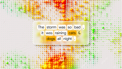 Gemma Scope: Google's Microscope for Peering into AI's Thought ProcessApr 17, 2025 am 11:55 AM
Exploring the Inner Workings of Language Models with Gemma Scope Understanding the complexities of AI language models is a significant challenge. Google's release of Gemma Scope, a comprehensive toolkit, offers researchers a powerful way to delve in
 Who Is a Business Intelligence Analyst and How To Become One?Apr 17, 2025 am 11:44 AM
Unlocking Business Success: A Guide to Becoming a Business Intelligence Analyst Imagine transforming raw data into actionable insights that drive organizational growth. This is the power of a Business Intelligence (BI) Analyst – a crucial role in gu
 How to Add a Column in SQL? - Analytics VidhyaApr 17, 2025 am 11:43 AM
SQL's ALTER TABLE Statement: Dynamically Adding Columns to Your Database In data management, SQL's adaptability is crucial. Need to adjust your database structure on the fly? The ALTER TABLE statement is your solution. This guide details adding colu
 Business Analyst vs. Data AnalystApr 17, 2025 am 11:38 AM
Introduction Imagine a bustling office where two professionals collaborate on a critical project. The business analyst focuses on the company's objectives, identifying areas for improvement, and ensuring strategic alignment with market trends. Simu
 What are COUNT and COUNTA in Excel? - Analytics VidhyaApr 17, 2025 am 11:34 AM
Excel data counting and analysis: detailed explanation of COUNT and COUNTA functions Accurate data counting and analysis are critical in Excel, especially when working with large data sets. Excel provides a variety of functions to achieve this, with the COUNT and COUNTA functions being key tools for counting the number of cells under different conditions. Although both functions are used to count cells, their design targets are targeted at different data types. Let's dig into the specific details of COUNT and COUNTA functions, highlight their unique features and differences, and learn how to apply them in data analysis. Overview of key points Understand COUNT and COU
 Chrome is Here With AI: Experiencing Something New Everyday!!Apr 17, 2025 am 11:29 AM
Google Chrome's AI Revolution: A Personalized and Efficient Browsing Experience Artificial Intelligence (AI) is rapidly transforming our daily lives, and Google Chrome is leading the charge in the web browsing arena. This article explores the exciti
 AI's Human Side: Wellbeing And The Quadruple Bottom LineApr 17, 2025 am 11:28 AM
Reimagining Impact: The Quadruple Bottom Line For too long, the conversation has been dominated by a narrow view of AI’s impact, primarily focused on the bottom line of profit. However, a more holistic approach recognizes the interconnectedness of bu
 5 Game-Changing Quantum Computing Use Cases You Should Know AboutApr 17, 2025 am 11:24 AM
Things are moving steadily towards that point. The investment pouring into quantum service providers and startups shows that industry understands its significance. And a growing number of real-world use cases are emerging to demonstrate its value out


Hot AI Tools

Undresser.AI Undress
AI-powered app for creating realistic nude photos

AI Clothes Remover
Online AI tool for removing clothes from photos.

Undress AI Tool
Undress images for free

Clothoff.io
AI clothes remover

AI Hentai Generator
Generate AI Hentai for free.

Hot Article

Hot Tools

SecLists
SecLists is the ultimate security tester's companion. It is a collection of various types of lists that are frequently used during security assessments, all in one place. SecLists helps make security testing more efficient and productive by conveniently providing all the lists a security tester might need. List types include usernames, passwords, URLs, fuzzing payloads, sensitive data patterns, web shells, and more. The tester can simply pull this repository onto a new test machine and he will have access to every type of list he needs.

PhpStorm Mac version
The latest (2018.2.1) professional PHP integrated development tool

DVWA
Damn Vulnerable Web App (DVWA) is a PHP/MySQL web application that is very vulnerable. Its main goals are to be an aid for security professionals to test their skills and tools in a legal environment, to help web developers better understand the process of securing web applications, and to help teachers/students teach/learn in a classroom environment Web application security. The goal of DVWA is to practice some of the most common web vulnerabilities through a simple and straightforward interface, with varying degrees of difficulty. Please note that this software

Dreamweaver Mac version
Visual web development tools

Dreamweaver CS6
Visual web development tools


