With the rapid development of deep reinforcement learning technology, more and more research teams have begun to apply it to autonomous driving decision planning, integrating behavioral decision-making with motion planning modules to directly learn driving trajectories.
The decision-making planning module in autonomous driving is one of the core indicators for measuring and evaluating autonomous driving capabilities. Its main task is to analyze the current environment after receiving various sensory information from sensors, and then Issue instructions to the underlying control module. A typical decision planning module can be divided into three levels: global path planning, behavioral decision-making, and motion planning.
01 Introduction
In a complete autonomous driving system, if the perception module is compared to human eyes and ears, then the decision-making planning is the brain of autonomous driving. After receiving various sensory information from the sensor, the brain analyzes the current environment and then issues instructions to the underlying control module. This process is the main task of the decision-making and planning module. At the same time, how complex scenarios the decision-making planning module can handle is also one of the core indicators for measuring and evaluating autonomous driving capabilities [1].
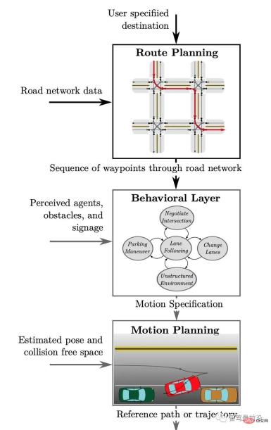
Figure 1. The hierarchical structure of the decision-making planning module in the autonomous driving system, quoted from [2]
As shown in Figure 1, a typical decision-making The planning module can be divided into three levels.
Among them, after receiving a given driving destination, the global route planning (Route Planning) combines the map information to generate a global route as a reference for subsequent specific route planning;
After receiving the global path, the behavioral decision-making layer combines the environmental information obtained from the perception module (including other vehicles and pedestrians, obstacles, and traffic rule information on the road) to make specific behavioral decisions (such as Choose to change lanes to overtake or follow);
Finally, based on specific behavioral decisions, the Motion Planning layer plans to generate a path that satisfies specific constraints (such as the dynamic constraints of the vehicle itself, collision avoidance, and passenger comfort). properties, etc.), which is used as the input of the control module to determine the final driving path of the vehicle.
This article will introduce the main functions and common algorithms of each layer respectively, and compare the advantages and disadvantages of various algorithms and applicable scenarios.
02 Global path planning (Route Planning)
Global path planning refers to selecting an optimal path through search after given the current position of the vehicle and the end target. The "optimal path" here is "Including conditions such as the shortest path or the fastest arrival time. This process is similar to the "navigation" function we often use in our lives. The difference is that the high-precision map used in autonomous driving is different from our common maps. The high-precision map contains more information about each lane. More information. Common global path planning algorithms include Dijkstra and A algorithms, as well as various improvements based on these two algorithms. Dijkstra's algorithm [3] and A* algorithm [4] are also the two most widely used search algorithms in many planning problems.
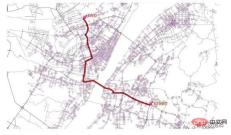
Figure 2. Global path planning diagram
1. Dijkstra algorithm
Dijkstra algorithm was developed by computer scientists Edsger W. Dijkstra proposed it in 1956 to find the shortest path between nodes in a graph. In Dijkstra's algorithm, the total movement cost of each node from the starting point needs to be calculated. At the same time, a priority queue structure is also needed. All nodes to be traversed will be sorted according to cost when placed in the priority queue. During the running of the algorithm, the node with the smallest cost is selected from the priority queue as the next traversed node each time. until you reach the end.
The advantage of Dijkstra's algorithm is that the path given is the optimal; the disadvantage is that the calculation time complexity is relatively high (O(N2)), because it explores the surroundings without a clear direction.
2. A* algorithm
In order to solve the search efficiency problem of Dijkstra algorithm, in 1968, the A algorithm was developed by Peter Hart, Nils Nilsson and Bertram Raphael of Stanford Research Institute. Published, its main improvement is to use a heuristic function to guide the search process. Specifically, Algorithm A calculates the priority of each node through the following function:
f(n)=g(n) h(n)
where:
- f(n) is the comprehensive priority of node n. When we select the next node to traverse, we always select the node with the highest overall priority (minimum value).
- g(n) is the cost of node n from the starting point.
- h(n) is the estimated cost of node n from the end point, which is the heuristic function of the A* algorithm.
03 Behavioral Layer
After determining the global path, the autonomous vehicle needs to make appropriate decisions based on specific road conditions, traffic rules, other vehicles and pedestrians, etc. behavioral decisions.
This process faces three main problems:
First, the real driving scenes are ever-changing, how to cover them?
Secondly, the real driving scene is a multi-agent decision-making environment. The behavior of each participant, including the main vehicle, will have an impact on other participants in the environment, so we It is necessary to predict the behavior of other participants in the environment;
Finally, it is impossible for autonomous vehicles to perceive 100% of environmental information, for example, there are many possible dangerous situations that are blocked by obstacles.
Based on the above points, in the autonomous driving behavior decision-making layer, what we need to solve is the planning problem of perceptual uncertainty in the complex environment of multi-agent decision-making. It can be said that this problem is one of the core bottlenecks in truly realizing L4 and L5 level autonomous driving technology. In recent years, with the rapid development of deep reinforcement learning and other fields, new ideas and dawn have been brought to solve this problem.
The models of the behavioral decision-making layer are divided into four categories and introduced separately [5]:
1. Finite state machine model
Autonomous driving vehicle The initial decision-making model is the finite state machine model [6]. The vehicle selects appropriate driving behaviors according to the current environment, such as parking, changing lanes, overtaking, avoidance, slow driving, etc. The state machine model constructs a finite directed connected graph. To describe different driving states and the transition relationships between states, so as to reactively generate driving actions based on the transition of driving states.
The finite state machine model is the most widely used behavioral decision-making model in the field of autonomous driving because of its simplicity and ease of implementation. However, this type of model ignores the dynamics and uncertainty of the environment. In addition, when the driving scene characteristics In many cases, the division and management of states are cumbersome and are mostly suitable for simple scenarios. It is difficult to perform behavioral decision-making tasks in urban road environments with rich structural features.
2. Decision tree model
The decision/behavior tree model [7] is similar to the state machine model. It also selects different parameters reactively through the attribute values of the current driving state. Driving actions, but the difference is that this type of model solidifies the driving status and control logic into a tree structure, and searches for driving strategies through a top-down "polling" mechanism. This type of decision-making model has visual control logic, and the control nodes can be reused, but it needs to define the decision-making network offline for each driving scenario. When the state space and behavior space are large, the control logic will be more complex. In addition, this type of model is also unable to consider the uncertainty factors existing in the traffic environment.
3. Knowledge-based reasoning and decision-making model
The knowledge-based reasoning and decision-making model imitates the behavior of human drivers by the mapping relationship of "scene characteristics-driving actions" Decision-making process, this type of model stores driving knowledge in a knowledge base or neural network. The driving knowledge here is mainly represented by the mapping relationship between rules, cases or scene features to driving actions. Then, driving actions are inferred from the knowledge base or trained network structure through the "query" mechanism.
This type of model mainly includes: rule-based reasoning system [8], case-based reasoning system [9] and neural network-based mapping model [10].
This type of model relies heavily on prior driving knowledge and training data, and requires careful organization, management, and updating of driving knowledge. Although the mapping model based on neural networks can omit data annotation and knowledge integration process, but there are still the following shortcomings:
- Its "data" driven mechanism makes it highly dependent on training data, and the training data needs to be sufficient [11];
- Solidifying the mapping relationship into the network structure has poor interpretability;
- has a "black box" problem and poor transparency. It has poor traceability for problems that occur in the actual system, and it is difficult to find the root cause of the problem. .
4. Value-based decision-making model
According to the maximum utility theory, the basic idea of the utility/value-based decision-making model is to select multiple criteria based on the selection criteria. Select the optimal driving strategy/action among alternatives [12].
In order to evaluate the quality of each driving action, this type of model defines a utility (utility) or value (value) function to quantitatively evaluate the degree to which the driving strategy meets the driving task objectives based on certain criterion attributes. For unmanned For driving tasks, these criterion attributes can be safety, comfort, driving efficiency, etc. Utility and value can be determined by a single attribute or multiple attributes.
Furda and Vlacic of Griffith University in Australia proposed a multi-criteria decision-making method to select the optimal driving action from the candidate action set [13]; Bandyopadhyay et al. of the National University of Singapore proposed a behavioral decision-making based on POMDP model [14] to solve situations where there is perceived uncertainty; Wei J and others from Carnegie Mellon University proposed a behavioral decision-making model [15] based on PCB (Prediction and-Cost-function Based), which focuses on It lies in how to construct an appropriate cost function to guide the prediction of the environment; in order to solve the decision-making problem in a complex environment involving multiple agents, many models based on game theory are also used by researchers to reason about the interaction between vehicles [16 ], [17]; in addition, due to its advantages in feature extraction, deep reinforcement learning technology has also begun to be widely used to complete the generation of optimal driving actions [18].
04 Motion Planning
After determining the specific driving behavior, what we need to do is to transform the "behavior" into a more specific driving "trajectory" so that we can finally Generate a series of specific control signals for the vehicle to achieve the vehicle's driving according to the planned target. This process is called motion planning. The concept of motion planning has a long history of research in the field of robotics. From a mathematical perspective, we can regard it as an optimization problem as follows:
Path Planning
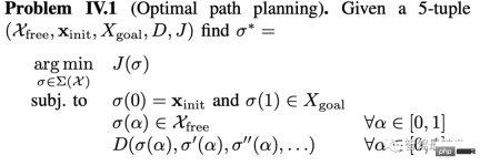
#Figure 3. Definition of path planning
In many scenarios represented by robots, We can think of our surroundings as certain. In this case, the so-called path planning refers to finding a mapping σ:[0,1]➞Χ that satisfies certain constraints in a given state space Χ. These constraints include:
- The determined starting state and the area where the target point is located
- Avoid collision
- Differential constraints on the path (for example, in actual problems, the path curvature cannot be too small, corresponding to its second-order Constraints on derivatives)
The objective functional of this optimization problem is defined as J(σ), and its specific meaning can be expressed as path length, control complexity and other measures.
However, in the automatic driving problem, the environment around the vehicle is constantly changing dynamically, so simple path planning cannot give a solution that is always valid during the driving process, so we need to add a dimension - time T , the corresponding planning problem is usually called trajectory planning.
Trajectory Planning
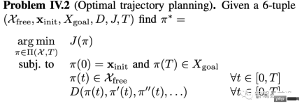
Figure 4. Definition of Trajectory Planning
Increase of time dimension poses a huge challenge to planning issues. For example, for a robot moving in a 2D environment, which is abstracted as a single point, the obstacles in the environment are approximated as polygons. The path planning problem can be solved in polynomial time, while the trajectory planning problem that adds the time dimension has been proven to be an NP-hard problem.
In the actual scenario of autonomous driving, whether it is the vehicle itself or the surrounding environment, establishing a more accurate model means more complex constraints on the optimization problem, and it also means that the solution is more difficult. Therefore, the algorithms actually used are based on the approximation of actual scenarios, and seek an optimal balance between model accuracy and solution efficiency.
The following introduces several common types of motion planning algorithms in the field of autonomous driving. In practice, it is often the combination of several types of ideas that can ultimately achieve better planning results and satisfy more different needs. Scenes.
1. Search-based planning algorithm
Solving motion planning problems through search is one of the simplest ideas. The basic idea is to pass the state space through a determined The method is discretized into a graph, and then various heuristic search algorithms are used to search for feasible solutions or even optimal solutions.
In the process of discretizing the state space, attention should be paid to ensuring that the final grid has the largest coverage area and does not repeat. As shown in Figure 5, the grid on the left is generated by three behaviors: go straight, turn left 90°, and turn right 90°; and if you choose three behaviors: go straight, turn left 89°, and turn right 89°, you will not be able to Generate a grid structure covering the entire area.
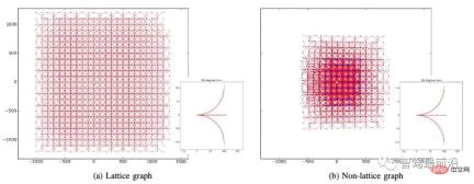
Figure 5. Constructing a raster graph, quoted from [2]
After rasterizing the state space, we can use Dijkstra, which has been introduced previously. A* search algorithm to complete the final planning. However, in actual complex environments, there are many grids and the environment changes dynamically over time, which will lead to too many search nodes. Therefore, a variety of improved algorithms have been developed to deal with different specific scenarios:
1) Hybrid A* algorithm, based on the A* algorithm, considers the maximum steering problem of the vehicle. For example, the maximum steering direction of the vehicle on the calculated path is limited to no more than 5°. The current application scenarios of this algorithm include car U-turns (the Junior car used by Stanford to participate in the DARPA challenge used this algorithm to perform uturn), parking and other scenarios that require high steering wheel control.
2) D* and D*Lite algorithms search from the end point to the starting point in advance, using the Dijkstra algorithm to store the shortest path length k from the target point to each point in the road network, and the shortest path length k from the node to the target point. The actual length value h, in the initial case k==h, and the previous node of each node is stored to ensure that the link can be followed.
After the calculation is completed, an optimal path at that time is obtained. When the car travels to a certain node and finds that the node is impassable (there are obstacles) through the sensor, the h value of some relevant points in the stored road network information is modified (increased), and a neighbor point is selected that still satisfies the problem. h==k, that is, the point on the optimal path is still the next point.
Then walk to the end. This type of algorithm is suitable for navigation and path planning in unknown environments, and is widely used in various current mobile robots and autonomous vehicles, such as the "Opportunity" and "Spirit" Mars rovers.
2. Sampling-based planning algorithm
By sampling the continuous state space, the original problem is approximated into a discrete sequence optimization problem. This idea It is also the most widely used algorithm in computer science. In motion planning problems, basic sampling-based algorithms include Probabilistic Roadmap (PRM) and Rapid Search Random Tree (RRT) algorithms.
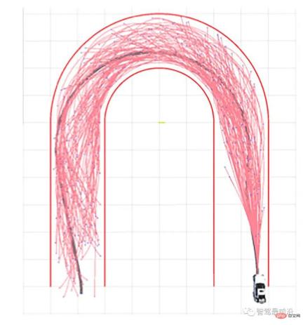
Figure 6. U-shaped curve trajectory planning using RRT algorithm, quoted from [19]
1) Basic algorithm: probabilistic route Figure (PRM)
- # Preprocessing stage: uniformly and randomly sample n points in the safe area in the state space, and each sampling point is connected to adjacent sampling points within a certain distance. Connect, and discard the trajectories that collide with obstacles, and finally obtain a connected graph.
- Query stage: For a given pair of initial and target states, connect them to the already constructed graph, and then use the search algorithm to find a trajectory that meets the requirements.
It is easy to see that once a PRM is constructed, it can be used to solve motion planning problems in different initial and target states, but this feature is unnecessary for autonomous driving motion planning. In addition, PRM requires precise connections between states, which is very difficult for motion planning problems with complex differential constraints.
2) Basic algorithm: Rapid Search Random Tree (RRT)
- Initialization of the tree: Initialize the node set and edge set of the tree, the node set Contains only the initial state, and the edge set is empty.
- Tree growth: Randomly sample the state space. When the sampling point falls in the safe area of the state space, select the node closest to the sampling point in the current tree and expand (or connect) it to the sampling point. If the generated trajectory does not collide with obstacles, the trajectory is added to the edge set of the tree, and the end point of the trajectory is added to the node set of the tree.
RRT is an incremental sampling search method that does not require setting any resolution parameters. In the extreme case, the search tree will densely cover the entire space. At this time, the search tree is composed of many shorter curves or paths to achieve the purpose of filling the entire space.
3) Various improved algorithms
From the description of the above basic algorithm, we can understand that sampling the state space can ensure that the starting point and the end point are connected. Feasible solution, but because the sampling process uniformly samples the entire space, the efficiency is very low; real-time solution cannot be achieved in complex scenarios; in addition, the final planning result cannot guarantee that the feasible solution obtained is the optimal solution. In response to these disadvantages, a variety of improved algorithms have been proposed and applied to autonomous driving problems:
- Efficiency improvement--uneven sampling
- RRT-Connect: build two Two trees start from the initial state and the target state respectively. When the two trees grow together, a feasible solution is found.
- Heuristic (hRRT): Use a heuristic function to increase the probability that nodes with low expansion costs are sampled.
- Combined with the driver model: Combined with the driver visual attention model for biased sampling, using visual feature information to guide motion planning, so that the planned trajectory is more consistent with human driving behavior.
- Construct a new metric RG-RRT (reachability guided RT): the conventional Euclidean distance metric cannot truly reflect the distance between configurations or states. RG-RRT calculates the reachability set of nodes in the tree , when the distance from the sampling point to the node is greater than the distance from the sampling point to the reachable set of the node, the node may be selected for expansion.
- Add obstacle penalty (RC-RRT, EG-RRT, ADD-RRT, etc.): Reduce the probability that nodes close to obstacles will be expanded.
- Real-time improvement
- anytime RRT first quickly builds an RRT, obtains a feasible solution and records its cost. After that, the algorithm will continue sampling, but it will only benefit Nodes that reduce the cost of feasible solutions are inserted into the tree, thereby gradually obtaining better feasible solutions.
- Replanning decomposes the entire planning task into a number of equal-time sub-task sequences, and plans the next task while executing the current task.
- Optimality improvement
- PRM*, RRG, RRT*: According to the random geometric graph theory (randomly sample m points in the state space, and divide the distance Points smaller than r(n) are connected to form a random geometric graph) The standard PRM and RRT are improved, and the PRM*, RRG and RRT* algorithms with asymptotic optimal properties are obtained
3. Direct optimization method
In most cases, regardless of height changes, the trajectory planning problem of autonomous driving is a three-dimensional constrained optimization problem (2D space time T). Therefore, We can use a decoupling strategy to decompose the original problem into several low-dimensional problems, thereby greatly reducing the difficulty of solving it.
1) Frenet coordinate system
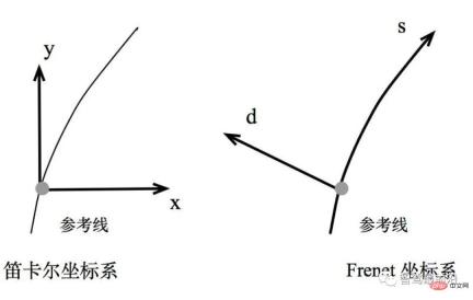
Figure 7. Frenet coordinate system
Due to the real world The roads in are all curved. In order to simplify the parameter expression of solving optimization problems, the Frenet coordinate system is usually used in autonomous driving.
In the Frenet coordinate system, we use the center line of the road as the reference line, and use the tangent vector t and normal vector n of the reference line to establish a coordinate system, as shown in the figure on the right, which takes the vehicle itself as The origin, the coordinate axes are perpendicular to each other, divided into the s direction (that is, the direction along the reference line, often called longitudinal, Longitudinal) and the d direction (or L direction, that is, the current normal direction of the reference line, called horizontal, Lateral ), compared to the Cartesian coordinate system (left picture), the Frenet coordinate system significantly simplifies the problem.
Because when driving on the road, we can always easily find the reference line of the road (i.e., the center line of the road), then the position based on the reference line can simply be expressed using the longitudinal distance S (i.e., along the It is described by the distance along the road direction) and the lateral distance L (that is, the distance away from the reference line).
2) Path-speed decoupling method
#In the Frenet coordinate system, the path-speed decoupling method optimizes the path and speed respectively. Path optimization mainly Considering static obstacles, a static reference path (SL dimension) is generated through dynamic planning, and then based on the generated path, speed planning (ST dimension) is considered. This process can be iterated continuously, enabling real-time updates to the trajectory. The EM planner used in Baidu's open source autonomous driving platform Apollo is based on a similar solution. This solution has strong flexibility and can be universally applied to many scenarios.
In addition, you can also choose different decoupling methods, such as planning the longitudinal trajectory (ST dimension) and transverse trajectory (LT dimension) separately. However, it should be pointed out that the solution obtained through the decoupling method may not be optimal, and this algorithm is not complete, and a feasible solution may not be found in some complex environments.
4. Parametric curve construction method

Figure 8. Common parametric curve construction method, quoted from [19]
The starting point of the parametric curve construction method is the constraints of the vehicle itself, including kinematics and dynamics constraints. Therefore, the generally planned path needs to have continuous curvature. This type of method considers obstacles based on the starting point and target point, and gives a smooth path by constructing a family of curves that conform to vehicle constraints.
As shown in Figure 8, common curves include Dubins curve (consisting of straight lines and arcs, which is the shortest curve family of a simple vehicle model Dubin model in two-dimensional space), clothoid curve, and polynomial curve , Bezier curve, spline curve, etc. It is difficult to simply apply the parametric curve construction method to meet actual complex scenarios. Therefore, more and more autonomous driving systems now combine it with other methods to smooth the planned and generated trajectories to satisfy vehicle kinematics and dynamics. Learn constraints.
5. Artificial potential field method
The artificial potential field method is inspired by the electromagnetic field in physics. It is assumed that obstacles and target positions generate repulsion and gravity respectively, so that the path can be planned along the fastest gradient descent of the potential field. A key issue in this type of method is how to select an appropriate potential field function. For example, Stephen Waydo uses flow functions for smooth path planning [20], and Robert Daily proposes a harmonic potential field path planning method on high-speed vehicles [21]. In simple scenarios, the artificial potential field method has high solution efficiency, but its biggest problem is that it may fall into a local minimum. In this case, the path obtained is not optimal, and the path may not even be found.
05 Algorithm complexity (Complexity)
In planning problems, in addition to considering its time and space complexity, the evaluation of an algorithm must also consider whether it has completeness and Optimality, take a step back and consider whether it has probabilistic completeness and asymptotic optimality. Only on the basis of understanding these properties can we design and apply different algorithms for different actual scenarios, so as to achieve the best balance between model complexity and optimal efficiency.
1) Completeness: If there is a path solution between the starting point and the target point, then the solution must be obtained. If the solution cannot be obtained, it must mean that there is no solution;
2) Probabilistically Completeness: If there is a path solution between the starting point and the target point, as long as the planning or search time is long enough, you will be sure to find a path solution;
3) Optimality: The planned path is optimal on a certain evaluation index (the evaluation index is generally the length of the path)
4) Asymptotically optimality: after a finite number of The path obtained after planning iterations is a suboptimal path that is close to the optimal, and it is closer to the optimal path after each iteration. It is a gradual convergence process

Table 1 Comparison of common algorithms
06 Future development trends

Figure 9. Autonomous driving development timeline and important motion planning algorithms in the process, quoted from [19 ]
Humanity’s interest in autonomous driving can be traced back to 1925. In recent years, the research boom on autonomous driving began with the U.S. Defense Advanced Research Projects Agency (DARPA) in 2004-2007. The 3rd Autonomous Driving Challenge held [22] is shown in Figure 9. After that, the effectiveness of the various decision-making planning methods mentioned above were actually verified. At the same time, solutions that combine motion planning methods with control theory, state parameter estimation, machine learning and other multi-field methods continue to emerge, becoming a future development trend:
1) Combined with vehicle dynamics: Combining dynamic parameter evaluation indicators with optimal planning, planning from the perspective of optimal control is a method often used in recent years. In this process, vehicle dynamics factors can be fully considered, and the planned trajectory is more reasonable. For example, use model predictive control theory (Model Predictive Control). The disadvantage is that the more constraints there are on the vehicle, the more difficult it is to optimize its trajectory, and it is more difficult to achieve online real-time calculation.
2) Combined with state parameter estimation: state parameter estimation can obtain vehicle parameters more accurately, so the state estimator can be added to the planning module to improve the trajectory by estimating the vehicle state online and feeding it back to the planner. quality. For example, different ground types will cause changes in vehicle slip characteristics, thereby affecting the vehicle status. By combining estimated parameters, the trajectory can be re-planned in real time and closed-loop planning can improve trajectory safety.
3) Combining with machine learning: With the rapid development of artificial intelligence represented by neural networks, many traditional planning problems have also brought new solutions. In the field of autonomous driving, its development trends include:
- End-to-end model: Use a deep neural network to derive the vehicle's control signal directly based on the vehicle status and external environment information. Although the current end-to-end model is uninterpretable like a "black box", it is believed that as humans continue to deepen their understanding of deep neural networks, this method has strong development potential due to its outstanding advantages of simplicity and efficiency.
- Integration of decision-making and motion planning modules
- Autonomous vehicles make optimal decisions in complex environments. This problem is very consistent with the definition of reinforcement learning. Therefore, as mentioned above, with depth With the rapid development of reinforcement learning technology, more and more research teams have begun to apply it to autonomous driving decision planning, integrating behavioral decision-making with motion planning modules to directly learn driving trajectories. In order to solve the problem that the environmental reward function is not easy to obtain, it has also been proposed to first use inverse reinforcement learning (IRL) to learn based on human expert demonstrations, and then use reinforcement learning to learn the optimal policy.
The above is the detailed content of Detailed explanation of autonomous driving decision planning technology. For more information, please follow other related articles on the PHP Chinese website!
 如何在 RHEL 9 上配置 DHCP 服务器Jun 08, 2023 pm 07:02 PM
DHCP是“动态主机配置协议DynamicHostConfigurationProtocol”的首字母缩写词,它是一种网络协议,可自动为计算机网络中的客户端系统分配IP地址。它从DHCP池或在其配置中指定的IP地址范围分配客户端。虽然你可以手动为客户端系统分配静态IP,但DHCP服务器简化了这一过程,并为网络上的客户端系统动态分配IP地址。在本文中,我们将演示如何在RHEL9/RockyLinux9上安装和配置DHCP服务器。先决条件预装RHEL9或RockyLinux9具有sudo管理权限的普
 在容器中怎么使用nginx搭建上传下载的文件服务器May 15, 2023 pm 11:49 PM
一、安装nginx容器为了让nginx支持文件上传,需要下载并运行带有nginx-upload-module模块的容器:sudopodmanpulldocker.io/dimka2014/nginx-upload-with-progress-modules:latestsudopodman-d--namenginx-p83:80docker.io/dimka2014/nginx-upload-with-progress-modules该容器同时带有nginx-upload-module模块和ng
 服务器怎么使用Nginx部署Springboot项目May 14, 2023 pm 01:55 PM
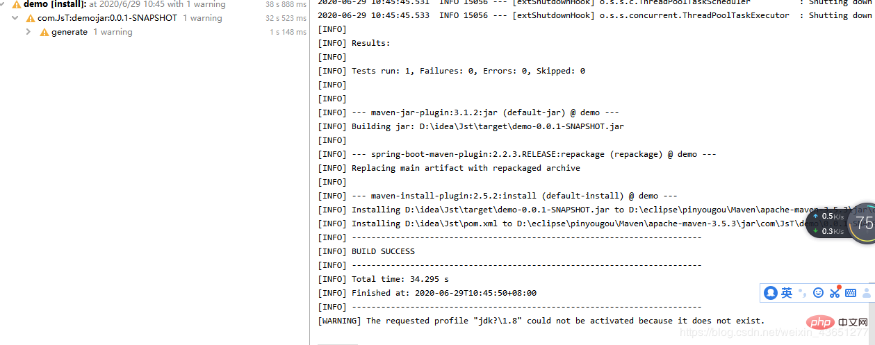
1,将java项目打成jar包这里我用到的是maven工具这里有两个项目,打包完成后一个为demo.jar,另一个为jst.jar2.准备工具1.服务器2.域名(注:经过备案)3.xshell用于连接服务器4.winscp(注:视图工具,用于传输jar)3.将jar包传入服务器直接拖动即可3.使用xshell运行jar包注:(服务器的java环境以及maven环境,各位请自行配置,这里不做描述。)cd到jar包路径下执行:nohupjava-jardemo.jar>temp.txt&
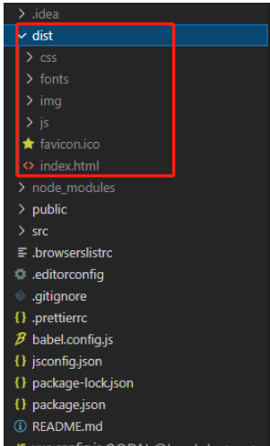 vue3项目打包发布到服务器后访问页面显示空白怎么解决May 17, 2023 am 08:19 AM
vue3项目打包发布到服务器后访问页面显示空白1、处理vue.config.js文件中的publicPath处理如下:const{defineConfig}=require('@vue/cli-service')module.exports=defineConfig({publicPath:process.env.NODE_ENV==='production'?'./':'/&
 python中怎么使用TCP实现对话客户端和服务器May 17, 2023 pm 03:40 PM
TCP客户端一个使用TCP协议实现可连续对话的客户端示例代码:importsocket#客户端配置HOST='localhost'PORT=12345#创建TCP套接字并连接服务器client_socket=socket.socket(socket.AF_INET,socket.SOCK_STREAM)client_socket.connect((HOST,PORT))whileTrue:#获取用户输入message=input("请输入要发送的消息:&
 Linux怎么在两个服务器直接传文件May 14, 2023 am 09:46 AM
scp是securecopy的简写,是linux系统下基于ssh登陆进行安全的远程文件拷贝命令。scp是加密的,rcp是不加密的,scp是rcp的加强版。因为scp传输是加密的,可能会稍微影响一下速度。另外,scp还非常不占资源,不会提高多少系统负荷,在这一点上,rsync就远远不及它了。虽然rsync比scp会快一点,但当小文件众多的情况下,rsync会导致硬盘I/O非常高,而scp基本不影响系统正常使用。场景:假设我现在有两台服务器(这里的公网ip和内网ip相互传都可以,当然用内网ip相互传
 如何使用psutil模块获取服务器的CPU、内存和磁盘使用率?May 07, 2023 pm 10:28 PM
psutil是一个跨平台的Python库,它允许你获取有关系统进程和系统资源使用情况的信息。它支持Windows、Linux、OSX、FreeBSD、OpenBSD和NetBSD等操作系统,并提供了一些非常有用的功能,如:获取系统CPU使用率、内存使用率、磁盘使用率等信息。获取进程列表、进程状态、进程CPU使用率、进程内存使用率、进程IO信息等。杀死进程、发送信号给进程、挂起进程、恢复进程等操作。使用psutil,可以很方便地监控系统的运行状况,诊断问题和优化性能。以下是一个简单的示例,演示如何
 怎么在同一台服务器上安装多个MySQLMay 29, 2023 pm 12:10 PM
一、安装前的准备工作在进行MySQL多实例的安装前,需要进行以下准备工作:准备多个MySQL的安装包,可以从MySQL官网下载适合自己环境的版本进行下载:https://dev.mysql.com/downloads/准备多个MySQL数据目录,可以通过创建不同的目录来支持不同的MySQL实例,例如:/data/mysql1、/data/mysql2等。针对每个MySQL实例,配置一个独立的MySQL用户,该用户拥有对应的MySQL安装路径和数据目录的权限。二、基于二进制包安装多个MySQL实例


Hot AI Tools

Undresser.AI Undress
AI-powered app for creating realistic nude photos

AI Clothes Remover
Online AI tool for removing clothes from photos.

Undress AI Tool
Undress images for free

Clothoff.io
AI clothes remover

AI Hentai Generator
Generate AI Hentai for free.

Hot Article

Hot Tools

ZendStudio 13.5.1 Mac
Powerful PHP integrated development environment

mPDF
mPDF is a PHP library that can generate PDF files from UTF-8 encoded HTML. The original author, Ian Back, wrote mPDF to output PDF files "on the fly" from his website and handle different languages. It is slower than original scripts like HTML2FPDF and produces larger files when using Unicode fonts, but supports CSS styles etc. and has a lot of enhancements. Supports almost all languages, including RTL (Arabic and Hebrew) and CJK (Chinese, Japanese and Korean). Supports nested block-level elements (such as P, DIV),

SecLists
SecLists is the ultimate security tester's companion. It is a collection of various types of lists that are frequently used during security assessments, all in one place. SecLists helps make security testing more efficient and productive by conveniently providing all the lists a security tester might need. List types include usernames, passwords, URLs, fuzzing payloads, sensitive data patterns, web shells, and more. The tester can simply pull this repository onto a new test machine and he will have access to every type of list he needs.

WebStorm Mac version
Useful JavaScript development tools

DVWA
Damn Vulnerable Web App (DVWA) is a PHP/MySQL web application that is very vulnerable. Its main goals are to be an aid for security professionals to test their skills and tools in a legal environment, to help web developers better understand the process of securing web applications, and to help teachers/students teach/learn in a classroom environment Web application security. The goal of DVWA is to practice some of the most common web vulnerabilities through a simple and straightforward interface, with varying degrees of difficulty. Please note that this software


