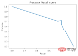
On the precision-recall curve, the same points are plotted with different coordinate axes. Warning: The first red dot on the left (0% recall, 100% precision) corresponds to 0 rules. The second dot on the left is the first rule, and so on.
Skope-rules uses a tree model to generate rule candidates. First build some decision trees and consider the paths from the root node to internal nodes or leaf nodes as rule candidates. These candidate rules are then filtered by some predefined criteria such as precision and recall. Only those with precision and recall above their thresholds are retained. Finally, similarity filtering is applied to select rules with sufficient diversity. In general, Skope-rules is applied to learn the underlying rules for each root cause.

Project address: https://github.com/scikit-learn-contrib/skope-rules
- Skope-rules is a build Python machine learning module on top of scikit-learn, released under the 3-clause BSD license.
- Skope-rules aims to learn logical, interpretable rules for "defining" a target category, that is, detecting instances of that category with high accuracy.
- Skope-rules are a trade-off between the interpretability of decision trees and the modeling capabilities of random forests.

schema
Installation
You can use pip to get the latest resources:
pip install skope-rules
Quick Start
SkopeRules can be used to describe classes with logical rules:
from sklearn.datasets import load_iris
from skrules import SkopeRules
dataset = load_iris()
feature_names = ['sepal_length', 'sepal_width', 'petal_length', 'petal_width']
clf = SkopeRules(max_depth_duplicatinotallow=2,
n_estimators=30,
precision_min=0.3 ,
recall_min=0.1,
feature_names=feature_names)
for idx, species in enumerate(dataset.target_names):
X, y = dataset.data, dataset.target
clf.fit(X, y == idx)
rules = clf.rules_[0:3]
print("Rules for iris", species)
for rule in rules:
print( rule)
print()
print(20*'=')
print()

Note:
If it appears The following error:

Solution:
About Python import error: cannot import name 'six' from 'sklearn.externals' , Yun Duojun on Stack Overflow Found a similar question on: https://stackoverflow.com/questions/61867945/
The solution is as follows
import six
import sys
sys.modules['sklearn .externals.six'] = six
import mlrose
Personal test is valid!
SkopeRules can also be used as predictors if using the "score_top_rules" method:
from sklearn.datasets import load_boston
from sklearn.metrics import precision_recall_curve
from matplotlib import pyplot as plt
from skrules import SkopeRules
dataset = load_boston()
clf = SkopeRules(max_depth_duplicatinotallow=None,
n_estimators=30,
precision_min=0.2,
recall_min=0.01 ,
feature_names=dataset.feature_names)
X, y = dataset.data, dataset.target > 25
X_train, y_train = X[:len(y)//2], y [:len(y)//2]
X_test, y_test = X[len(y)//2:], y[len(y)//2:]
clf.fit(X_train, y_train )
y_score = clf.score_top_rules(X_test) # Get a risk score for each test example
precision, recall, _ = precision_recall_curve(y_test, y_score)
plt.plot(recall, precision)
plt.xlabel('Recall')
plt.ylabel('Precision')
plt.title('Precision Recall curve')
plt.show()

Practical Case
This case demonstrates the use of skope-rules on the famous Titanic data set.
skope-rules Applicability:
- Solving two-classification problems
- Extracting interpretable decision rules
This case is divided into 5 parts
- Import related libraries
- Data preparation
- Model training (using ScopeRules().score_top_rules() method)
- Explanation of "Survival Rules" (using SkopeRules().rules_property).
- Performance analysis (using SkopeRules.predict_top_rules() method).
Import related libraries
# Import skope-rules
from skrules import SkopeRules
# Import librairies
import pandas as pd
from sklearn.ensemble import GradientBoostingClassifier, RandomForestClassifier
from sklearn.model_selection import train_test_split
from sklearn.tree import DecisionTreeClassifier
import matplotlib.pyplot as plt
from sklearn.metrics import roc_curve, precision_recall_curve
from matplotlib import cm
import numpy as np
from sklearn.metrics import confusion_matrix
from IPython.display import display
# Import Titanic data
data = pd.read_csv('../ data/titanic-train.csv')
Data preparation
# Delete rows with missing ages
data = data.query('Age == Age')
# is The variable Sex creates an encoded value
data['isFemale'] = (data['Sex'] == 'female') * 1
# The variable Embarked creates an encoded value
data = pd.concat(
[data,
pd.get_dummies(data.loc[:,'Embarked'],
dummy_na=False,
prefix='Embarked',
prefix_sep='_')],
axis=1
)
# Delete unused variables
data = data.drop(['Name', 'Ticket', 'Cabin',
'PassengerId', 'Sex ', 'Embarked'],
axis = 1)
# Create training and test sets
X_train, X_test, y_train, y_test = train_test_split(
data.drop(['Survived'], axis =1),
data['Survived'],
test_size=0.25, random_state=42)
feature_names = X_train.columns
print('Column names are: ' ' '. join(feature_names.tolist()) '.')
print('Shape of training set is: ' str(X_train.shape) '.')
Column names are: Pclass Age SibSp Parch Fare
isFemale Embarked_C Embarked_Q Embarked_S.
Shape of training set is: (535, 9).
Model training
# Train a gradient boosting classifier for benchmark testing
gradient_boost_clf = GradientBoostingClassifier(random_state=42, n_estimators=30, max_depth = 5)
gradient_boost_clf.fit(X_train, y_train)
# Train a random forest classifier for benchmarking
random_forest_clf = RandomForestClassifier(random_state=42, n_estimators=30, max_depth = 5)
random_forest_clf.fit(X_train, y_train)
# Train a decision tree classifier for benchmarking
decision_tree_clf = DecisionTreeClassifier(random_state=42, max_depth = 5)
decision_tree_clf.fit(X_train, y_train)
# Train a skope-rules-boosting classifier
skope_rules_clf = SkopeRules(feature_names=feature_names, random_state= 42, n_estimators=30,
recall_min=0.05, precision_min=0.9,
max_samples=0.7,
max_depth_duplicatinotallow= 4, max_depth = 5)
skope_rules_clf.fit(X_train, y_train)
# Calculate prediction score
gradient_boost_scoring = gradient_boost_clf.predict_proba(X_test)[:, 1]
random_forest_scoring = random_forest_clf.predict_proba(X_test)[:, 1]
decision_tree_scoring = decision_tree_clf.predict_proba( X_test)[:, 1]
skope_rules_scoring = skope_rules_clf.score_top_rules(X_test)
Extraction of "Survival Rules"
# Get the number of created survival rules
print("Created with SkopeRules" str(len(skope_rules_clf.rules_)) "rules n")
# Print these rules
rules_explanations = [
"Under 3 years old and under 37 years old , women in first or second class. "
"Females over 3 years old traveling in first or second class and paying more than 26 euros. "
"Female who travels in first or second class and pays more than 29 euros. "
"Female who is over 39 years old and traveling in first or second class. "
]
print('The four best-performing "Titanic survival rules" are as follows:/n')
for i_rule, rule in enumerate(skope_rules_clf.rules_[:4] )
print(rule[0])
print('->' rules_explanations[i_rule] 'n')
9 rules were created using SkopeRules.
Among them The top 4 "Titanic Survival Rules" are as follows:
Age 2.5
and Pclass 0.5
-> Women under 3 years old and under 37 years old, in first or second class.
Age > 2.5 and Fare > 26.125
and Pclass 0.5
-> Women over 3 years old traveling in first or second class and paying more than 26 euros.
Fare > 29.356250762939453
and Pclass 0.5
-> Women who ride in first or second class and pay more than 29 euros.
Age > 38.5 and Pclass and isFemale > 0.5
-> Women who are over 39 years old and traveling in first or second class.
def compute_y_pred_from_query(X, rule):
score = np.zeros(X.shape[0])
X = X.reset_index(drop=True)
score[list( X.query(rule).index)] = 1
return(score)
def compute_performances_from_y_pred(y_true, y_pred, index_name='default_index'):
df = pd.DataFrame(data=
{
'precision':[sum(y_true * y_pred)/sum(y_pred)],
'recall':[sum(y_true * y_pred)/sum(y_true)]
},
index=[index_name],
columns=['precision', 'recall']
)
return(df)
def compute_train_test_query_performances(X_train, y_train, X_test, y_test , rule):
y_train_pred = compute_y_pred_from_query(X_train, rule)
y_test_pred = compute_y_pred_from_query(X_test, rule)
performances = None
performances = pd.concat([
performances,
compute_performances_from_y_pred(y_train, y_train_pred, 'train_set')],
axis=0)
performances = pd.concat([
performances,
compute_performances_from_y_pred(y_test, y_test_pred, ' test_set')],
axis=0)
return(performances)
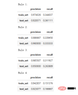
print('Precision = 0.96 means that 96% of the people determined by the rules are survivors. ')
print('Recall = 0.12 means that the survivors identified by the rule account for 12% of the total number of survivors n')
for i in range(4):
print('Rule ' str (i 1) ':')
display(compute_train_test_query_performances(X_train, y_train,
X_test, y_test,
skope_rules_clf.rules_[i][0])
)
Precision = 0.96 means that 96% of the people determined by the rules are survivors.
Recall = 0.12 means that the survivors identified by the rule account for 12% of the total survivors.

Model performance detection
def plot_titanic_scores(y_true, scores_with_line=[], scores_with_points=[],
labels_with_line=['Gradient Boosting', 'Random Forest', 'Decision Tree'],
labels_with_points=['skope-rules']):
gradient = np.linspace(0, 1, 10)
color_list = [ cm .tab10(x) for x in gradient ]
fig, axes = plt.subplots(1, 2, figsize=(12, 5),
sharex=True, sharey=True)
ax = axes[0]
n_line = 0
for i_score, score in enumerate(scores_with_line):
n_line = n_line 1
fpr, tpr, _ = roc_curve(y_true, score)
ax.plot(fpr, tpr, linestyle='-.', c=color_list[i_score], lw=1, label=labels_with_line[i_score])
for i_score, score in enumerate(scores_with_points):
fpr , tpr, _ = roc_curve(y_true, score)
ax.scatter(fpr[:-1], tpr[:-1], c=color_list[n_line i_score], s=10, label=labels_with_points[i_score] )
ax.set_title("ROC", fnotallow=20)
ax.set_xlabel('False Positive Rate', fnotallow=18)
ax.set_ylabel('True Positive Rate (Recall)', fnotallow =18)
ax.legend(loc='lower center', fnotallow=8)
ax = axes[1]
n_line = 0
for i_score, score in enumerate(scores_with_line ):
n_line = n_line 1
precision, recall, _ = precision_recall_curve(y_true, score)
ax.step(recall, precision, linestyle='-.', c=color_list[i_score], lw =1, where='post', label=labels_with_line[i_score])
for i_score, score in enumerate(scores_with_points):
precision, recall, _ = precision_recall_curve(y_true, score)
ax.scatter (recall, precision, c=color_list[n_line i_score], s=10, label=labels_with_points[i_score])
ax.set_title("Precision-Recall", fnotallow=20)
ax.set_xlabel('Recall (True Positive Rate)', fnotallow=18)
ax.set_ylabel('Precision', fnotallow=18)
ax.legend(loc='lower center', fnotallow=8)
plt.show ()
plot_titanic_scores(y_test,
scores_with_line=[gradient_boost_scoring, random_forest_scoring, decision_tree_scoring],
scores_with_points=[skope_rules_scoring]
)

On the ROC curve, each red point corresponds to the number of activated rules (from skope-rules). For example, the lowest point is the result point of 1 rule (the best). The second lowest point is the 2 rule result point, and so on.
On the precision-recall curve, the same points are plotted with different coordinate axes. Warning: The first red dot on the left (0% recall, 100% precision) corresponds to 0 rules. The second dot on the left is the first rule, and so on.
Some conclusions can be drawn from this example.
- skope-rules perform better than decision trees.
- The performance of skope-rules is similar to random forest/gradient boosting (in this example).
- Using 4 rules can achieve very good performance (61% recall, 94% precision) (in this example).
n_rule_chosen = 4
y_pred = skope_rules_clf.predict_top_rules(X_test, n_rule_chosen)
print('The performances reached with ' str(n_rule_chosen) ' discovered rules are the following: ')
compute_performances_from_y_pred(y_test, y_pred, 'test_set')

predict_top_rules(new_data, n_r) method is used to calculate the prediction of new_data, including the first n_r items skope-rules rules.
The above is the detailed content of Increase your knowledge! Machine learning with logical rules. For more information, please follow other related articles on the PHP Chinese website!
 Gemma Scope: Google's Microscope for Peering into AI's Thought ProcessApr 17, 2025 am 11:55 AM
Exploring the Inner Workings of Language Models with Gemma Scope Understanding the complexities of AI language models is a significant challenge. Google's release of Gemma Scope, a comprehensive toolkit, offers researchers a powerful way to delve in
 Who Is a Business Intelligence Analyst and How To Become One?Apr 17, 2025 am 11:44 AM
Unlocking Business Success: A Guide to Becoming a Business Intelligence Analyst Imagine transforming raw data into actionable insights that drive organizational growth. This is the power of a Business Intelligence (BI) Analyst – a crucial role in gu
 How to Add a Column in SQL? - Analytics VidhyaApr 17, 2025 am 11:43 AM
SQL's ALTER TABLE Statement: Dynamically Adding Columns to Your Database In data management, SQL's adaptability is crucial. Need to adjust your database structure on the fly? The ALTER TABLE statement is your solution. This guide details adding colu
 Business Analyst vs. Data AnalystApr 17, 2025 am 11:38 AM
Introduction Imagine a bustling office where two professionals collaborate on a critical project. The business analyst focuses on the company's objectives, identifying areas for improvement, and ensuring strategic alignment with market trends. Simu
 What are COUNT and COUNTA in Excel? - Analytics VidhyaApr 17, 2025 am 11:34 AM
Excel data counting and analysis: detailed explanation of COUNT and COUNTA functions Accurate data counting and analysis are critical in Excel, especially when working with large data sets. Excel provides a variety of functions to achieve this, with the COUNT and COUNTA functions being key tools for counting the number of cells under different conditions. Although both functions are used to count cells, their design targets are targeted at different data types. Let's dig into the specific details of COUNT and COUNTA functions, highlight their unique features and differences, and learn how to apply them in data analysis. Overview of key points Understand COUNT and COU
 Chrome is Here With AI: Experiencing Something New Everyday!!Apr 17, 2025 am 11:29 AM
Google Chrome's AI Revolution: A Personalized and Efficient Browsing Experience Artificial Intelligence (AI) is rapidly transforming our daily lives, and Google Chrome is leading the charge in the web browsing arena. This article explores the exciti
 AI's Human Side: Wellbeing And The Quadruple Bottom LineApr 17, 2025 am 11:28 AM
Reimagining Impact: The Quadruple Bottom Line For too long, the conversation has been dominated by a narrow view of AI’s impact, primarily focused on the bottom line of profit. However, a more holistic approach recognizes the interconnectedness of bu
 5 Game-Changing Quantum Computing Use Cases You Should Know AboutApr 17, 2025 am 11:24 AM
Things are moving steadily towards that point. The investment pouring into quantum service providers and startups shows that industry understands its significance. And a growing number of real-world use cases are emerging to demonstrate its value out


Hot AI Tools

Undresser.AI Undress
AI-powered app for creating realistic nude photos

AI Clothes Remover
Online AI tool for removing clothes from photos.

Undress AI Tool
Undress images for free

Clothoff.io
AI clothes remover

AI Hentai Generator
Generate AI Hentai for free.

Hot Article

Hot Tools

SecLists
SecLists is the ultimate security tester's companion. It is a collection of various types of lists that are frequently used during security assessments, all in one place. SecLists helps make security testing more efficient and productive by conveniently providing all the lists a security tester might need. List types include usernames, passwords, URLs, fuzzing payloads, sensitive data patterns, web shells, and more. The tester can simply pull this repository onto a new test machine and he will have access to every type of list he needs.

Safe Exam Browser
Safe Exam Browser is a secure browser environment for taking online exams securely. This software turns any computer into a secure workstation. It controls access to any utility and prevents students from using unauthorized resources.

Atom editor mac version download
The most popular open source editor

MinGW - Minimalist GNU for Windows
This project is in the process of being migrated to osdn.net/projects/mingw, you can continue to follow us there. MinGW: A native Windows port of the GNU Compiler Collection (GCC), freely distributable import libraries and header files for building native Windows applications; includes extensions to the MSVC runtime to support C99 functionality. All MinGW software can run on 64-bit Windows platforms.

Dreamweaver CS6
Visual web development tools


