


There are some very classic function combinations in Excel. The more familiar ones are the INDEX-MATCH combination and the INDEX-SMALL-IF-ROW combination (also called the Tiger Balm combination). Of course, there are many other combinations. The combination shared today is also very useful. Below, we will use four common questions to let everyone witness the wonderful moments brought by this combination. Of course, we still need to get to know today’s two protagonists first: COUNTIF and IF are two functions that everyone is very familiar with.
How to use the COUNTIF function: COUNTIF (range, condition), the function can get the number of times that data that meets the conditions appears in the range. Simply put, this function is used for conditional counting;
Usage of the IF function: IF (condition, result that satisfies the condition, result that does not satisfy the condition), in one sentence, if you give IF a condition (the first parameter), when the condition is established, it will return a result (the second parameter) parameter), when the condition is not met, another result is returned (the third parameter).
Regarding the basic usage of these two functions, I have talked about them many times in previous tutorials, so I won’t go into details again. Let’s take a look at the first problem that occurred after the two of them met: the problems encountered when checking orders.
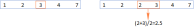
Assume that column A is all the order numbers, and column D is the order number that has been shipped. Now you need to mark the shipped orders in column B (to prevent everyone from being confused, the arrows only point out two Corresponding order number):

I think you must be familiar with this question. It is often used during reconciliation. Some friends may not be able to wait. I shouted VLOOKUP. In fact, the formula in column B is like this: =IF(COUNTIF(D:D,A2)>0,"shipped","")

First use COUNTIF to make statistics and see how many times the order number in cell A2 appears in column D. If it does not appear, it means it has not been shipped, otherwise it means it has been shipped.
So use COUNTIF(D:D,A2)>0 as the condition of IF. If the order appears in column D (the number of occurrences is greater than 0), then return "shipped" " (note that Chinese characters must be enclosed in quotation marks), otherwise a blank will be returned (two quotation marks represent a blank).
Now that you understand the first question, let’s look at the second question: COUNTIF to check duplicate cases: how to find duplicate orders
Column A is an order statistics table registered by multiple clerks , after summarizing, it is found that some are duplicates (for the convenience of viewing, you can sort the order numbers first), now you need to mark the duplicate orders in column B:

This is also a problem with a very high ranking rate, and the solution is also very simple. The formula in column B is: =IF(COUNTIF(A:A,A2)>1,"Yes","")

Similar to the previous question, this time we directly calculate the number of times each order appears in column A, but the conditions need to be changed. It is not greater than 0 but greater than 1. , this is also easy to understand. Only those with occurrence times greater than 1 are duplicate orders, so use COUNTIF(A:A,A2)>1 as the condition, and then let IF return the results we need.
When duplicate orders are found, the third question arises. You need to specify whether to keep the information after the order number. If there are duplicates, keep one:

This problem may seem troublesome at first glance. In fact, it can be achieved by slightly modifying the formula for question 2: =IF(COUNTIF($A$2:A2,A2)=1,"Keep" ,"")

Note that the range of COUNTIF here is no longer the entire column, but $A$2:A2, this way of writing As the formula is pulled down, the statistical range will change, and the result is as follows:

It is not difficult to see that the order numbers with a result of 1 are all the order numbers that appear for the first time. , is also the information we need to retain, so when used as a condition, it is equal to 1.
The first three questions are all related to the order number, and the last question is related to the supplier assessment. This is the key issue that determines whether the contract can be renewed.
According to company regulations, there are six assessment indicators for each supplier. A is the best and E is the worst. If there are two or more E's in the six indicators, the contract will not be renewed. :

The rules are relatively simple. Let’s see if the formula is equally simple: =IF(COUNTIF(B2:G2,"E")>1,"No" ,"")

This time the range of COUNTIF changes to rows. Count the number of occurrences of "E" in the range B2:G2. Pay attention to the same Add quotation marks. When the statistical result is greater than 1, it means that the supplier has more than two negative reviews (if you insist on using greater than or equal to 2, I have no objection), and then use IF to get the final result.
The last question I want to talk about must be familiar to partners in financial positions. Sometimes we will encounter this situation: there is a positive and a negative situation in a column of data. At this time, the unoffset data needs to be Mark (extract) it, such as the example in the picture:

# This problem may have caused a headache to many people, but in fact it can be easily solved using today’s combination of these two functions. , the formula is: =IF(COUNTIF(A:A,-A2)=0,A2,"")

Note here that in COUNTIF Condition-A2, that is, find a number that can cancel each other out with A2. If not, get A2 through IF. Otherwise, get a null value. Using a negative sign cleverly solves a troublesome problem.
Through the above five cases, you may have a feeling that the combination of these two functions is relatively easier to understand than some other function combinations. As long as you find the right idea, this combination can be used for many problems. to handle. This is also true. If you are good at using COUNTIF to count various conditions, and then use the IF function to get more diverse results, ifcountif is often used to filter duplicate data. Solving problems does not necessarily require difficult functions. It is also very pleasant to use simple functions well.
Related learning recommendations: excel tutorial
The above is the detailed content of How to use the countif() function in Excel function learning. For more information, please follow other related articles on the PHP Chinese website!

 MEDIAN formula in Excel - practical examplesApr 11, 2025 pm 12:08 PM
This tutorial explains how to calculate the median of numerical data in Excel using the MEDIAN function. The median, a key measure of central tendency, identifies the middle value in a dataset, offering a more robust representation of central tenden
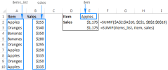
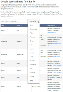
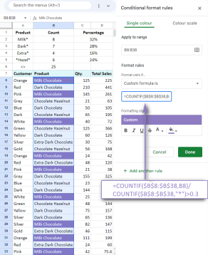 Google Spreadsheet COUNTIF function with formula examplesApr 11, 2025 pm 12:03 PM
Master Google Sheets COUNTIF: A Comprehensive Guide This guide explores the versatile COUNTIF function in Google Sheets, demonstrating its applications beyond simple cell counting. We'll cover various scenarios, from exact and partial matches to han
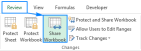 Excel shared workbook: How to share Excel file for multiple usersApr 11, 2025 am 11:58 AM
This tutorial provides a comprehensive guide to sharing Excel workbooks, covering various methods, access control, and conflict resolution. Modern Excel versions (2010, 2013, 2016, and later) simplify collaborative editing, eliminating the need to m
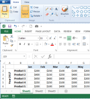 How to convert Excel to JPG - save .xls or .xlsx as image fileApr 11, 2025 am 11:31 AM
This tutorial explores various methods for converting .xls files to .jpg images, encompassing both built-in Windows tools and free online converters. Need to create a presentation, share spreadsheet data securely, or design a document? Converting yo
 Excel names and named ranges: how to define and use in formulasApr 11, 2025 am 11:13 AM
This tutorial clarifies the function of Excel names and demonstrates how to define names for cells, ranges, constants, or formulas. It also covers editing, filtering, and deleting defined names. Excel names, while incredibly useful, are often overlo
 Standard deviation Excel: functions and formula examplesApr 11, 2025 am 11:01 AM
This tutorial clarifies the distinction between standard deviation and standard error of the mean, guiding you on the optimal Excel functions for standard deviation calculations. In descriptive statistics, the mean and standard deviation are intrinsi
 Square root in Excel: SQRT function and other waysApr 11, 2025 am 10:34 AM
This Excel tutorial demonstrates how to calculate square roots and nth roots. Finding the square root is a common mathematical operation, and Excel offers several methods. Methods for Calculating Square Roots in Excel: Using the SQRT Function: The
 Google Sheets basics: Learn how to work with Google SpreadsheetsApr 11, 2025 am 10:23 AM
Unlock the Power of Google Sheets: A Beginner's Guide This tutorial introduces the fundamentals of Google Sheets, a powerful and versatile alternative to MS Excel. Learn how to effortlessly manage spreadsheets, leverage key features, and collaborate


Hot AI Tools

Undresser.AI Undress
AI-powered app for creating realistic nude photos

AI Clothes Remover
Online AI tool for removing clothes from photos.

Undress AI Tool
Undress images for free

Clothoff.io
AI clothes remover

Video Face Swap
Swap faces in any video effortlessly with our completely free AI face swap tool!

Hot Article
Hot Tools

SublimeText3 Linux new version
SublimeText3 Linux latest version

SublimeText3 Mac version
God-level code editing software (SublimeText3)

MantisBT
Mantis is an easy-to-deploy web-based defect tracking tool designed to aid in product defect tracking. It requires PHP, MySQL and a web server. Check out our demo and hosting services.

VSCode Windows 64-bit Download
A free and powerful IDE editor launched by Microsoft

EditPlus Chinese cracked version
Small size, syntax highlighting, does not support code prompt function

