Practical Excel skills sharing: How to divide a column into multiple rows and columns?

To be honest, some people print out a form with many pages, but each page only occupies one side of the paper. Do you really have the courage to show such a document to your boss? It is ugly and a waste of paper. , you may get scolded bloody! Today, this article will share with you a tutorial on how to change an Excel table from one column to multiple columns. Why not hurry up and learn~

Sometimes there is only one column of data in our table. If you need to print it out, it will look like this:

Not only is it a waste of paper, it is also ugly.

For such data, Excel needs to divide a column into multiple rows and columns. There are usually two methods to achieve this. Let’s take a look at the operation method first:

1 , Operation method is to divide a long column of data into multiple columns

Step 1:First design the number of columns that need to be split, and then manually create the title;

In this example, we plan to split 8 columns.

Step 2: Enter a2 in cell c2, pull to the right, and Excel will automatically fill in a9 for us.

Step 3: Enter a10 in cell c3 and pull to the right; because the first row has reached a9, this row starts with a10 , filled until a17.

Step 4:Select two rows and pull them down together. Assuming there are 160 data, 8 in each row, then 20 rows are enough to drop down;

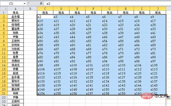
Step 5: Press the Ctrl h key combination to open Find and Replace. The search content is a and the replacement content is =a, as shown in the figure below;

Click Replace All, OK, and complete the operation.

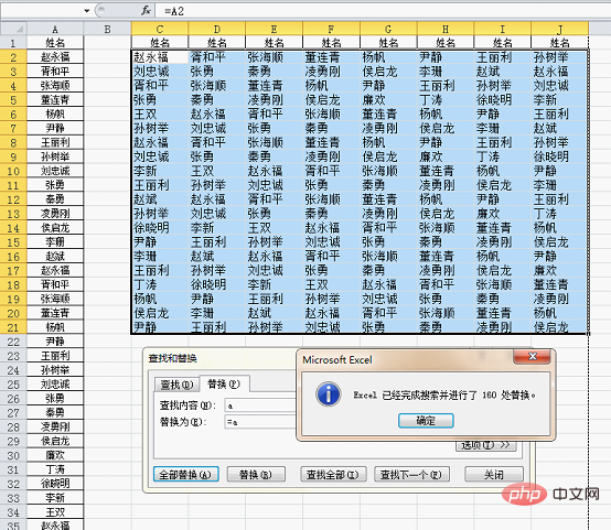
Step 6:Paste selectively as value to delete the formula, center the data with a border, set print preview, the effect is exactly what we need;

Conclusion:

1. If there are not 8 per row, you only need to adjust the number of the first right pull. ;

2. The advantage of the operation method is that it is easy to get started and is more suitable for novices;

3. However, the operation method also has shortcomings. If the data continues to increase, then it is quite necessary to do this every time. Troublesome, so you still need to know how to use formulas to divide an Excel column into multiple rows and columns.

2. Formula method to change one column of data into multiple columns

Let’s use this example to illustrate, usually changing one column into multiple columns will Using the OFFSET function, let's first take a look at what the formula looks like:

=OFFSET($A$1,MOD(COLUMN(A1) 7,8) ROW(A1)*8-7 ,)

#Just drag this formula to the right and pull it down.

OFFSET This function gets a new reference (cell or area) based on the offset. There are five parameters in total. The format is:

OFFSET (starting position, row offset, column offset, height, width).

In this example, the starting position is cell A1, because the data sources are all in one column, and they are all cell references, so you only need to determine the row offset, and you can see the formula Only two parameters are used, the second parameter is

MOD(COLUMN(A1) 7,8) ROW(A1)*8-7.

The effect of displaying this part alone is as follows:

To put it simply, A1 is 1 line, 2 lines down...etc. cell reference.

This part requires some basic knowledge of sequence construction. If you don’t understand it, you can remember the routine. If you want to learn how to construct a sequence, you can leave a message. We will explain how to construct a sequence in a formula separately.

Conclusion:

1. If there are not 8 per line, you only need to adjust the numbers 7 and 8 in the second parameter accordingly, for example, each line is 6 For data, the formula is modified to: =OFFSET($A$1,MOD(COLUMN(A1) 5,6) ROW(A1)*6-5,)

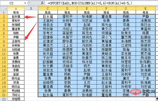
2. The formula method requires users to have certain experience. It is very flexible to adjust when the data source changes and has strong scalability.

Seeing this, some partners may be thinking: What if the data source is not one column, but two or three columns?

In fact, two-column or three-column data sources are more common in daily work, such as the following situation:

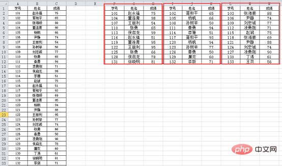
The data source has three columns , we hope to become nine columns (three groups), so that it is very reasonable to print. Have you learned how to divide a column of data into multiple columns in Excel introduced above?

For this kind of problem, it is more difficult to use the techniques introduced in Method 1. It is better to use the OFFSET function to deal with it.

3. Processing method for multi-column data sources

The formula is: =OFFSET($A$1,INT(COLUMN (C1)/3) ROW(A1)*3-3,MOD(COLUMN(C1),3))

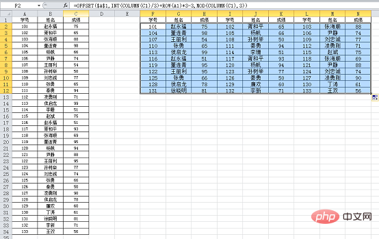
Because the data source is not in the same column , so the row offset and column offset must be considered, so three parameters are used. The starting position of the first parameter is still A1;

The second parameterINT(COLUMN(C1)/ 3) ROW(A1)*3-3 represents the row offset of the reference data relative to the starting position A1. Looking at it alone, the effect is:

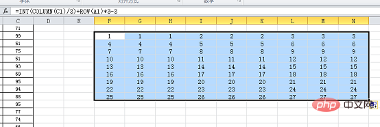
Okay You can see the change pattern very clearly;

The third parameter MOD(COLUMN(C1),3) represents the column offset of the reference data relative to the starting position A1. The effect of looking at it alone is:

The ability to control this pattern determines the level of use of the OFFSET function. It is precisely for this reason that many beginners are confused about the OFFSET function and never get the point when learning it. .

Our main purpose today is not to learn the OFFSET function, but to learn an application of this function. In this case, write down the routine of the formula, and then you can modify the formula according to your actual problem and solve the problem. enough.

The key to learning OFFSET well lies in the construction of the second and third parameters.

For example, in the above question, the data source is three columns and I want it to be four groups (twelve columns). The second parameter needs to be INT(COLUMN(C1)/3) ROW(A1) *4-4

Modify the two places pointed by the arrows.

The third parameter =MOD(COLUMN(C1),3) does not need to be adjusted; and so on, as long as the number of columns in the data source remains unchanged, only the above mentioned Two positions will do.

When the data source becomes 2 columns, the second parameter needs to be modified to INT(COLUMN(B1)/2) ROW(A1)*3-3

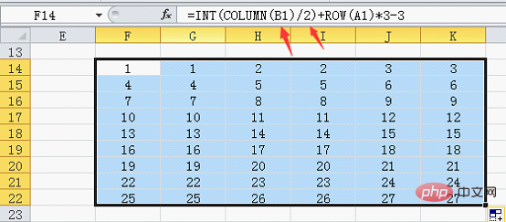
Still modify two positions, C is changed to B, 3 is changed to 2,

At the same time, the third parameter column offset also needs to be modified:

=MOD(COLUMN(B1),2)

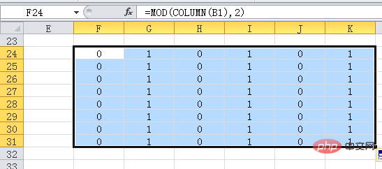
also modify two places, C is changed to B, and 3 is changed to 2.

By analogy, if the data source becomes 4 columns, modify B to D and 2 to 4 respectively.

Through the above explanation, you can basically understand how to adjust the corresponding content of the formula according to actual needs. If you want to fully understand the mystery here, the construction method of the sequence is an obstacle that cannot be bypassed. I hope this article’s tips for changing one column into multiple columns in Excel can be helpful to your work.

Let’s work together to learn those interesting and practical skills in Excel!

Related learning recommendations: excel tutorial

The above is the detailed content of Practical Excel skills sharing: How to divide a column into multiple rows and columns?. For more information, please follow other related articles on the PHP Chinese website!