 Topics
 excel
excel Practical Excel skills sharing: help you understand 'absolute reference' and 'mixed reference'
Practical Excel skills sharing: help you understand 'absolute reference' and 'mixed reference'
In the previous article " Practical Excel skills sharing: learn how to make a multi-factor ranking statistical table? 》, we learned about how to make a multi-factor ranking statistical table, and today we are going to talk about citations in Excel formulas. Don’t you understand absolute citations and mixed citations? No wonder you always fill in the wrong formulas!
Let me analyze this question for you.

After reading everyone’s comments, I found that there is a common problem with everyone’s formulas: the first parameter of each nested IF function uses the AND function to specify the data. range.
For example:

Also like this:

No matter whether the above formula is Correct, think about it, do we need to write so many ANDs?
Perhaps everyone was influenced by the tutorial - who said this tutorial just exemplified the AND function, and who said the subsidy years could just be described by AND? Haha...
(In the last question, due to the carelessness of the bottle, I forgot to write down the subsidy for more than 10 years! I will punish myself by writing more tutorials, so now we will unify that the subsidy for more than 10 years is also 600) There are two ways to write the
formula. The first one is:
=IF(C:C
When the number in column C is less than 1, return 0, otherwise Just look at the second IF directly. At this time, the default is greater than or equal to 1, so the second IF only needs to write the upper limit of the number, which is less than 2. The following is the same.
The above formula limits all upper limits. In fact, it can also limit all lower limits. The second type:
=IF(C:C>=8,600,IF(C:C> ;=6,400,IF(C:C>=4,300,IF(C:C>=2,200,IF(C:C>=1,100,0)))))
When column C When the number is greater than or equal to 8, it returns 600, when it is greater than or equal to 6, it returns 400, when it is greater than or equal to 4, it returns 300, when it is greater than or equal to 2, it returns 200, when it is greater than or equal to 1, it returns 100, otherwise it returns 0.
You can find that if you use IF to answer this question, use the second method and set the lower limit of the data every time, which is easier to understand.
In addition, Bo Bo also wants to tell you that when entering formulas in the edit bar, sometimes you don’t have to enter them manually. For example, in the above formula, we directly click on column number C, and it will appear in the formula. C:C. The formula written by the second friend above uses absolute reference. You can also directly drag and select the data area B5-B14 and press F4, and it will become $B$5:$B$14.
Maybe those who are just getting started don’t know much about relative references and absolute references. Today Bottle will explain them to you.
1. Relative reference
As shown below, the data in columns A and B are summed, and the summation result is displayed in column C. .

As shown below, after selecting cell C9, enter the equal sign in the edit bar, then directly click on cell A9, enter the plus sign, and then directly click on cell B9. Finally enter.

Select cell C9, place the mouse in the lower right corner, double-click, and you can see that the entire column has been summed.

At this time, we click on the cells in column C one by one, and we can see the formula in the edit bar. As we move down, the row number will also change. Change to the corresponding line number.


You can try entering the formula in cell A18, summing column A, and drag the fill formula horizontally to cell C18. . You will see that when you drag the formula horizontally, the column number will automatically change to the corresponding column number. This is called a relative reference. The relative reference format of a cell is the column number and row number. For example, A10, B14, etc. are all relative references. The biggest feature of relative references is that when you drag to fill in a formula, the cell will automatically change based on the location of the formula.
2. Absolute reference
What is an absolute reference?
As shown in the figure below, select cell D9, enter =sum(), click in the square brackets, directly drag to select A9-C9, then press F4, and finally press Enter.

At this time, double-click to fill in the formula, and then click on each cell in column D to view the formula. You will find that the formulas in the entire column are exactly the same. What is the difference between

and relative reference? The difference is that the row number and column number referenced in the current formula are preceded by the "$" symbol. $ is a "lock" that locks the cell, so no matter we pull it horizontally or vertically, the formula will not change in any way. This is called an absolute reference.
3. Mixed Reference
In the previous formula, the row number and column number are both "locked", but think about it, When filling in the formula vertically, the column number will not change even if we do not lock the column number.
As shown below, in cell E9, after entering =sum(), click in the square brackets, drag and select the cell range A9-C9, and then press F4 twice. At this time, only the rows are locked. Number.

After double-clicking to fill down, you can see that the result is exactly the same as the previous absolute reference result.

This kind of operation that only locks the row number or column number is called a mixed reference. Mixed means that cell references include both absolute references and relative references. For example, $A1 means that the column number of the cell is an absolute reference and the row number is a relative reference. The trick to mixed references is: pull down to lock only the row number, and pull to the right to lock only the column number. This way the formula will not change during the dragging process.
It’s time to verify everyone’s learning results!
Look at the table below. The corresponding columns and rows need to be displayed in cells B2-E5. The bottle has set the formula in cell B2. Now think about it, in the formula How to "lock" the row number and column number so that the entire area can be filled in at once?

Leave your answer in the comment area below!
Related learning recommendations: excel tutorial
The above is the detailed content of Practical Excel skills sharing: help you understand 'absolute reference' and 'mixed reference'. For more information, please follow other related articles on the PHP Chinese website!
 Excel RANK function and other ways to calculate rankApr 09, 2025 am 11:35 AM
This Excel tutorial details the nuances of the RANK functions and demonstrates how to rank data in Excel based on multiple criteria, group data, calculate percentile rank, and more. Determining the relative position of a number within a list is easi
 Capitalize first letter in Excel cellsApr 09, 2025 am 11:31 AM
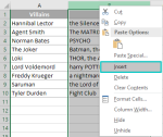
Three ways to convert the first letter of Excel cell When processing text data in Excel, a common requirement is to capitalize the first letter of a cell. Whether it is a name, product name, or task list, you may encounter some (or even all) cases where letters are inconsistent. Our previous article discussed the PROPER function, but it capitalizes the initial letter of each word in the cell and the other letters lowercase, so not all cases apply. Let's see what other options are available through an example of my favorite villain list. Use formula to capitalize the initial letter The first letter is capitalized, the remaining letters are lowercase Capitalize the initial letter, ignore the remaining letters Using the text toolbox: "Change case" Use public
 Complete guide to Google Sheets conditional formatting: rules, formulas, use casesApr 09, 2025 am 10:57 AM
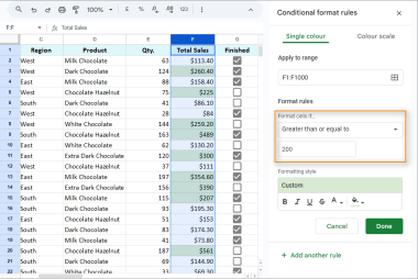
Master Google Sheets Conditional Formatting: A Comprehensive Guide This guide provides a complete walkthrough of Google Sheets' conditional formatting, from basic rules to advanced custom formulas. Learn how to highlight key data, save time, and red
 Google Sheets basics: share, move and protect Google SheetsApr 09, 2025 am 10:34 AM
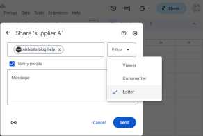
Mastering Google Sheets Collaboration: Sharing, Moving, and Protecting Your Data This "Back to Basics" guide focuses on collaborative spreadsheet management in Google Sheets. Learn how to efficiently share, organize, and protect your data
 Custom Data Validation in Excel : formulas and rulesApr 09, 2025 am 10:24 AM
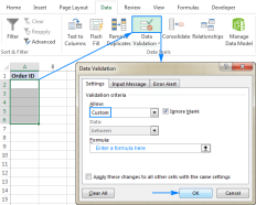
This tutorial demonstrates how to create custom data validation rules in Excel. We'll explore several examples, including formulas to restrict input to numbers, text, text starting with specific characters, unique entries, and more. Yesterday's tuto
 Google Sheets basics: edit, print and download the files in Google SheetsApr 09, 2025 am 10:09 AM
This "Back to Basics" guide delves into essential Google Sheets editing techniques. We'll cover fundamental actions like data deletion and formatting, and then move on to more advanced features such as comments, offline editing, and change
 Calculating time in Google SheetsApr 09, 2025 am 09:43 AM
Mastering Google Sheets Time Calculations: A Comprehensive Guide This guide delves into the intricacies of time calculations within Google Sheets, covering time differences, addition/subtraction, summation, and date/time extraction. Calculating Time
 How to use IFERROR in Excel with formula examplesApr 09, 2025 am 09:37 AM
This tutorial demonstrates how Excel's IFERROR function handles errors, replacing them with blanks, alternative values, or custom messages. It covers using IFERROR with VLOOKUP and INDEX MATCH, and compares it to IF ISERROR and IFNA. "Give me a


Hot AI Tools

Undresser.AI Undress
AI-powered app for creating realistic nude photos

AI Clothes Remover
Online AI tool for removing clothes from photos.

Undress AI Tool
Undress images for free

Clothoff.io
AI clothes remover

AI Hentai Generator
Generate AI Hentai for free.

Hot Article

Hot Tools

mPDF
mPDF is a PHP library that can generate PDF files from UTF-8 encoded HTML. The original author, Ian Back, wrote mPDF to output PDF files "on the fly" from his website and handle different languages. It is slower than original scripts like HTML2FPDF and produces larger files when using Unicode fonts, but supports CSS styles etc. and has a lot of enhancements. Supports almost all languages, including RTL (Arabic and Hebrew) and CJK (Chinese, Japanese and Korean). Supports nested block-level elements (such as P, DIV),

SublimeText3 Linux new version
SublimeText3 Linux latest version

MantisBT
Mantis is an easy-to-deploy web-based defect tracking tool designed to aid in product defect tracking. It requires PHP, MySQL and a web server. Check out our demo and hosting services.

SublimeText3 Chinese version
Chinese version, very easy to use

Safe Exam Browser
Safe Exam Browser is a secure browser environment for taking online exams securely. This software turns any computer into a secure workstation. It controls access to any utility and prevents students from using unauthorized resources.


