


This article brings you relevant knowledge about excel. It mainly introduces how to add serial numbers after filtering, multiply after filtering, and count according to conditions after filtering. Let’s take a look at it together. I hope it helps everyone.

Related learning recommendations: excel tutorial
1. Add the serial number after filtering
as shown in the figure below, To maintain continuous serial numbers in the filtered state, we can cancel the filter first, enter the following formula in cell D2, and then pull down:
=SUBTOTAL(3,E$1:E2)-1

The SUBTOTAL function only counts visible cell contents.
Using 3 for the first parameter indicates the calculation rule for executing the COUNTA function, that is, counting the number of visible cells for the second parameter.
The second parameter uses a dynamically expanded range E$1:E2. As the formula is pulled down, this range will become E$1:E3, E$1:E4, E$1:E5,...
The formula always calculates the number of visible non-empty cells in the area from the first row of column E to the row where the formula is located. Subtract 1 from the result, and the calculated result will be the same as the serial number, and it will remain continuous after filtering.
Note, please note that if this formula is changed to =SUBTOTAL(3,E$2:E2), that is, starting from the row where the formula is located, the serial number result will be fine, but the last row will be filtered by Excel. Always displayed as a summary row.
2. Multiply after filtering
As shown in the figure below, after filtering column E, you need to calculate the total amount multiplied by the unit price.
The formula in cell E2 is:
=SUMPRODUCT(SUBTOTAL(3,OFFSET(E3,ROW(1:13),))*F4:F16*G4:G16)

To calculate the filtered product, the key to the problem is to determine whether the data is visible.
How to judge this visible status?
Need to combine OFFSET and SUBTOTAL functions.
First use the OFFSET function, taking cell E3 as the base point, and offset rows 1 to 13 downwards in order to obtain a multi-dimensional reference. This multi-dimensional reference contains 13 reference areas with one row and one column, that is, individual cells from E4 to E16 are referenced respectively.
Next use the SUBTOTAL function, use 3 as the first parameter, that is, count the number of visible cells in each cell from E4 to E16 in sequence. If the cell is in the display state, count this cell. The result is 1, otherwise the statistical result is 0. Get a memory array with the following effect:
{1;0;1;1;1;1;0;0;1;1;0;1;0}
Use the above again The result is multiplied by the quantity in column F and the unit price in column G. If the cell is in the display state, it is equivalent to 1*quantity*unit price, otherwise it is equivalent to 0*quantity*unit price.
Finally use the SUMPRODUCT function to sum the products.
3. Count according to conditions after filtering
As shown in the figure below, after filtering the departments in column E, the number of people with more than 3 years of service must be calculated.
The formula in cell E2 is:
=SUMPRODUCT(SUBTOTAL(3,OFFSET(E3,ROW(1:13),))*(G4:G16>3))

The first half of the calculation principle is the same as the previous example, and the core is to determine whether the cell is visible.
The statistical conditions in the second half of the formula (G4:G16>3) are multiplied by the judgment results in the first half, indicating that both conditions are met at the same time, that is, the number of items in the visible state and column G is greater than 3 .
4. Automatically correct the title after filtering
As shown in the figure below, after filtering the department name in column E, you want the title of cell D1 to automatically change to the corresponding department name. The formula is:
=LOOKUP(1,0/SUBTOTAL(3,OFFSET(D1,ROW(1:15)-1,)),E:E)&”Statistics Table”

The combination of SUBTOTAL and OFFSET functions still aims to determine whether the cells in column D are visible. Get a memory array composed of 0 and 1:
{0;1;0;0;0;0;1;1;1;1;0;1;0;1;0}
Use the memory array 0/ to get a new memory array composed of 0 and error value:
{#DIV/0!;0;#DIV/0!…;0;0;0 ;0;#DIV/0!;0;#DIV/0!;0;#DIV/0!}
The LOOKUP function uses 1 as the query value to find the position of the last 0 in the above memory array , and returns the contents of column E at the corresponding position.
The ultimate goal is to extract the content of the last displayed cell after filtering.
Connect the extracted content with "statistical table" and turn it into an automatically updated table title.
Related learning recommendations: excel tutorial
The above is the detailed content of Calculation summary in Excel filtering state. For more information, please follow other related articles on the PHP Chinese website!

 MEDIAN formula in Excel - practical examplesApr 11, 2025 pm 12:08 PM
This tutorial explains how to calculate the median of numerical data in Excel using the MEDIAN function. The median, a key measure of central tendency, identifies the middle value in a dataset, offering a more robust representation of central tenden
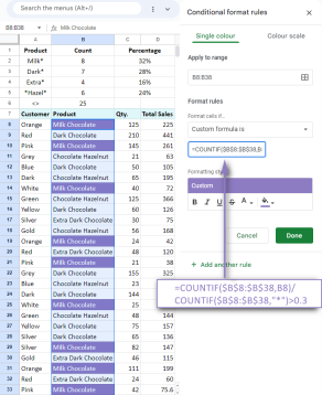 Google Spreadsheet COUNTIF function with formula examplesApr 11, 2025 pm 12:03 PM
Master Google Sheets COUNTIF: A Comprehensive Guide This guide explores the versatile COUNTIF function in Google Sheets, demonstrating its applications beyond simple cell counting. We'll cover various scenarios, from exact and partial matches to han
 Excel shared workbook: How to share Excel file for multiple usersApr 11, 2025 am 11:58 AM
This tutorial provides a comprehensive guide to sharing Excel workbooks, covering various methods, access control, and conflict resolution. Modern Excel versions (2010, 2013, 2016, and later) simplify collaborative editing, eliminating the need to m
 How to convert Excel to JPG - save .xls or .xlsx as image fileApr 11, 2025 am 11:31 AM
This tutorial explores various methods for converting .xls files to .jpg images, encompassing both built-in Windows tools and free online converters. Need to create a presentation, share spreadsheet data securely, or design a document? Converting yo
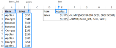 Excel names and named ranges: how to define and use in formulasApr 11, 2025 am 11:13 AM
This tutorial clarifies the function of Excel names and demonstrates how to define names for cells, ranges, constants, or formulas. It also covers editing, filtering, and deleting defined names. Excel names, while incredibly useful, are often overlo
 Standard deviation Excel: functions and formula examplesApr 11, 2025 am 11:01 AM
This tutorial clarifies the distinction between standard deviation and standard error of the mean, guiding you on the optimal Excel functions for standard deviation calculations. In descriptive statistics, the mean and standard deviation are intrinsi
 Square root in Excel: SQRT function and other waysApr 11, 2025 am 10:34 AM
This Excel tutorial demonstrates how to calculate square roots and nth roots. Finding the square root is a common mathematical operation, and Excel offers several methods. Methods for Calculating Square Roots in Excel: Using the SQRT Function: The
 Google Sheets basics: Learn how to work with Google SpreadsheetsApr 11, 2025 am 10:23 AM
Unlock the Power of Google Sheets: A Beginner's Guide This tutorial introduces the fundamentals of Google Sheets, a powerful and versatile alternative to MS Excel. Learn how to effortlessly manage spreadsheets, leverage key features, and collaborate


Hot AI Tools

Undresser.AI Undress
AI-powered app for creating realistic nude photos

AI Clothes Remover
Online AI tool for removing clothes from photos.

Undress AI Tool
Undress images for free

Clothoff.io
AI clothes remover

AI Hentai Generator
Generate AI Hentai for free.

Hot Article
Hot Tools

Atom editor mac version download
The most popular open source editor

MinGW - Minimalist GNU for Windows
This project is in the process of being migrated to osdn.net/projects/mingw, you can continue to follow us there. MinGW: A native Windows port of the GNU Compiler Collection (GCC), freely distributable import libraries and header files for building native Windows applications; includes extensions to the MSVC runtime to support C99 functionality. All MinGW software can run on 64-bit Windows platforms.

EditPlus Chinese cracked version
Small size, syntax highlighting, does not support code prompt function

Dreamweaver Mac version
Visual web development tools

Notepad++7.3.1
Easy-to-use and free code editor

