Detailed graphic explanation of typical usage of XLOOKUP function in Excel

This article brings you relevant knowledge about excel, which mainly introduces the relevant knowledge about the XLOOKUP function, including regular query, reverse query, returning multiple columns, automatic debugging and Let’s take a look at approximate search and other contents. I hope it will be helpful to everyone.

Related learning recommendations: excel tutorial

Today I would like to share with you some typical uses of the XLOOKUP function.

This function can currently only be used in Office 365 and WPS 2021. The function syntax is:

=XLOOKUP(search value, search range, result range, [fault tolerance value], [Matching method], [Query mode])

The first three parameters are required, and the following parameters can be omitted.

Next, let’s take a look at some typical uses of this function:

1. Regular query

As shown in the figure below, according to the department of G1, in column A Query the department and return the name of the corresponding person in column B. The formula is:

=XLOOKUP(G1,A2:A11,B2:B11)

The first parameter is the query content , the second parameter is the query area, and you only need to select one column for the query area. The third parameter is the content of which column to return, and you only need to select one column.

The meaning of the formula is to find the department specified in cell G1 in the cell range A2:A11, and return the corresponding name in the cell range B2:B11.

2. Reverse query

Since the query area and return area of ​​the XLOOKUP function are two separate parameters, there is no need to consider the direction of the query. Not only can it be achieved from left to right, You can also query in any direction from right to left, bottom to top, top to bottom, etc.

As shown in the figure below, according to the department of G1, query the department in column B and return the name of the person in charge corresponding to column A. The formula is:

=XLOOKUP(G1,B2:B11,A2:A11)

3. Return multiple columns

If you want to return the content in different columns based on the specified query content, it is also very simple.

As shown in the figure below, according to the department of cell G1, the name, date and sales amount corresponding to the department are returned. The formula is:

=XLOOKUP(G1,A2:A11,B2:D11)

The third parameter in this formula selects the range of multiple columns. Since the formulas in Office 365 have an overflow function, as long as you enter a formula, you can return multiple pieces of information in columns B~D.

4. Automatic debugging

The XLOOKUP function also comes with Shuanghuanglian. When the content cannot be queried, you can specify the prompt information to be returned.

As shown below, the XLOOKUP function cannot query the "Daxing Store" in cell G1 in column A. At this time, as long as you add a parameter, the formula will no longer return the error value #N/A.

=XLOOKUP(G1,A2:A11,B2:D11,"No such data")

The fourth parameter is used to specify when the result cannot be found The content of the returned prompt.

5. Approximate search

As shown below, according to the taxable income in cell F1, query the corresponding estimate in the comparison table on the left Discount rates and quick calculation deductions. The formula is:

=XLOOKUP(F2,B2:B8,C2:D8,0,-1)

XLOOKUP queries the value of F2 in column B, No. Use -1 for the five parameters, which means that if it cannot be found, return the next smaller value from the query area.

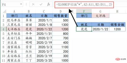
If the fifth parameter is 1, if the query value cannot be found, the next larger value in the query area will be returned.

Another cool thing about this usage is that the query area does not need to be sorted in advance. For example, in the table below, the values ​​in column B are out of order:

If wildcards are used in the query value, remember to select 2 for the fifth parameter.

The XLOOKUP function also has a sixth parameter. If there are two qualified results in the data source, the sixth parameter is set to 1 to return the first result. Set to -1 returns the last result.

Related learning recommendations: excel tutorial

The above is the detailed content of Detailed graphic explanation of typical usage of XLOOKUP function in Excel. For more information, please follow other related articles on the PHP Chinese website!