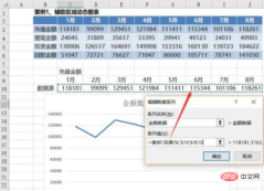
When using Excel for data analysis, you often need to draw data charts. Good charts can make people’s eyes brighter, and dynamic charts can better reflect the style and let your data display. Take it up a notch!
There are the following 3 methods for drawing dynamic charts in Excel.
1. Create an auxiliary area through sumifs to implement dynamic charts
2. Implement dynamic charts through offset and custom names
3. Implement dynamic charts through offset and development controls
Introduced below.
Create an auxiliary area through sumifs to realize dynamic charts
The effect is as follows:

Drawing method:
1. Set the selection sequence
Select cell C8, select the menu: Data-Data Verification-Data Verification, open the "Data Verification" window:
Allow : Selection sequence, source: Select the area indicated by the red box in the upper left corner

After the setting is completed, the selection sequence appears in cell C8:

2. Define the data source - use the sumifs formula
Copy the month to the bottom and define the data source through the formula sumifs.
Data source:


excel basic tutorial"
The specific operations to beautify charts are as follows: (1) Select a chart style


1. Set the selection sequence
The method is the same as step 1 of "Establishing an auxiliary area through sumifs formula to implement dynamic charts".
2. Define the data source - through the offset formula and custom name
Idea: First obtain the downward offset through match, and then reference the data source area through offset.
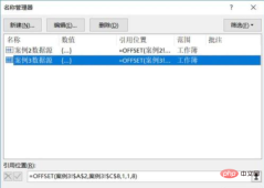
 Select menu: Formula-Name Manager
 Create a new name "Case 2 Data Source" and enter the following formula :
=OFFSET(Case 2!$B$2,MATCH(Case 2!$C$9,Case 2!$B$3:$B$6,0),1,1,8)
 3. Insert a bar chart, quote the data source, and beautify the chart
After inserting the bar chart, quote the data source method:
=Excel Dynamic drawing preparation. Renderings.

Achieving dynamic charts through offset formulas and development controls
The effect is as follows:

Drawing method :
1. Insert a radio control and set the control cell link
Select menu: Development Tools-Insert-Form Control, insert a radio control, and change the name to Recharge Amount

#Right-click the control and set the control cell link. Here, select cell C8.

Insert 3 more radio controls and modify the names: cash withdrawal amount, investment amount and repayment amount.

After the setting is completed, you can see that when you select different radio controls, the numbers in cell C8 will change, corresponding to 1, 2, 3, and 4 respectively.
2. Define the data source - through the offset formula and custom name
Idea: Use the offset formula and the number in the C8 unit to reference the data area.
Specific formula: =OFFSET(Case 3!$A$2,Case 3!$C$8,1,1,8)

Summary
This article introduces three ways to draw Excel dynamic charts: (1) Create an auxiliary area through sumifs to implement dynamic charts(2) Implement dynamic charts through offset and custom names(3) Implement dynamic charts through offset and development controlsThe above is the detailed content of What are the 3 ways to implement dynamic charts in Excel?. For more information, please follow other related articles on the PHP Chinese website!

Hot AI Tools

Undresser.AI Undress
AI-powered app for creating realistic nude photos

AI Clothes Remover
Online AI tool for removing clothes from photos.

Undress AI Tool
Undress images for free

Clothoff.io
AI clothes remover

Video Face Swap
Swap faces in any video effortlessly with our completely free AI face swap tool!

Hot Article

Hot Tools

SublimeText3 Mac version
God-level code editing software (SublimeText3)

Dreamweaver CS6
Visual web development tools

WebStorm Mac version
Useful JavaScript development tools

PhpStorm Mac version
The latest (2018.2.1) professional PHP integrated development tool

mPDF
mPDF is a PHP library that can generate PDF files from UTF-8 encoded HTML. The original author, Ian Back, wrote mPDF to output PDF files "on the fly" from his website and handle different languages. It is slower than original scripts like HTML2FPDF and produces larger files when using Unicode fonts, but supports CSS styles etc. and has a lot of enhancements. Supports almost all languages, including RTL (Arabic and Hebrew) and CJK (Chinese, Japanese and Korean). Supports nested block-level elements (such as P, DIV),


