Python implements LR classic algorithm

The example in this article describes the implementation of LR classic algorithm in Python. Share it with everyone for your reference, the details are as follows:

(1) Understanding the Logistic Regression (LR) classifier

First of all, although Logistic regression has "regression" in its name, it is actually a classification method, mainly used for two-classification problems. It uses the Logistic function (or Sigmoid function), and the independent variable value range is ( -INF, INF), the value range of the independent variable is (0,1), and the function form is:

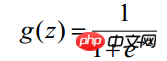
Because the domain of the sigmoid function is (-INF, INF), and the value range is (0, 1). Therefore, the most basic LR classifier is suitable for classifying two categories (class 0, class 1) targets. The Sigmoid function is a very beautiful "S" shape, as shown in the following figure:

LR classifier ( The purpose of Logistic Regression Classifier is to learn a 0/1 classification model from the training data features - this model uses the linear combination of the sample features as the independent variable, and uses the logistic function to map the independent variable to (0,1). Therefore, the solution of the LR classifier is to solve a set of weights ( is a nominal variable--dummy, which is a constant. In actual engineering, x0=1.0 is often used. Regardless of whether the constant term is meaningful or not, it is best to retain it), And substitute it into the Logistic function to construct a prediction function:

The value of the function represents the probability that the result is 1, which means that the feature belongs to The probability of y=1. Therefore, the probabilities that the input x classification result is category 1 and category 0 are respectively:

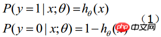
##When we want to determine which class a new feature belongs to, we can find a z value according to the following formula:

(x1,x2,...,xn are the characteristics of a certain sample data, and the dimension is n)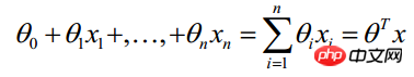

And then find out---If it is greater than 0.5, it is Class y=1, otherwise it belongs to class y=0. (Note: It is still assumed that the statistical samples are uniformly distributed, so the threshold is set to 0.5). How to obtain this set of weights of the LR classifier? This requires the concepts of maximum likelihood estimation (MLE) and optimization algorithms. The most commonly used optimization algorithm in mathematics is the gradient ascent (descent) algorithm.

Logistic regression can also be used for multi-class classification, but binary classification is more commonly used and easier to explain. Therefore, the most commonly used method in practice is binary logistic regression. The LR classifier is suitable for data types: numerical and nominal data. Its advantage is that the calculation cost is not high and it is easy to understand and implement; its disadvantage is that it is easy to underfit and the classification accuracy may not be high.

(2) Mathematical derivation of logistic regression

1, gradient descent method to solve logistic regression

First of all, understanding the following mathematical derivation process requires more derivative solution formulas. You can refer to "Commonly used basic elementary function derivation formulas and integral formulas".

Assume that there are n observation samples, and the observation values ​​are Let be the probability of obtaining yi=1 under given conditions. The conditional probability of getting yi=0 under the same conditions is . Therefore, the probability of obtaining an observed value is

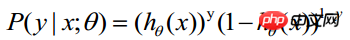-----This formula is actually a comprehensive formula (1) to get

Because each observation is independent, their joint distribution can be expressed as the product of each marginal distribution:

## (m represents the number of statistical samples) 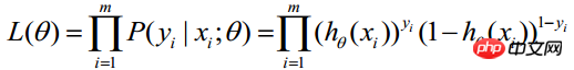                                                    #The above formula is called the likelihood function of n observations. Our goal is to be able to find parameter estimates that maximize the value of this likelihood function. Therefore, the key to maximum likelihood estimation is to find the parameters

so that the above formula obtains the maximum value.

Find the logarithm of the above function:

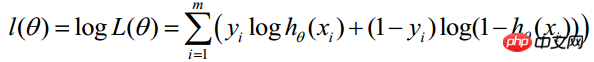
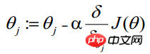
##Maximum likelihood estimation is to find θ when the above formula takes the maximum value. Here you can use the gradient ascent method to solve it. The obtained θ is the required optimal parameter. In Andrew Ng's course, J(θ) is taken as the following formula, that is: J(θ)=-(1/m)l(θ), and θ when J(θ) is at its minimum is the required optimal parameter. . Find the minimum value by gradient descent method. The initial values ​​of θ can all be 1.0, and the update process is:

(j represents the j-th attribute of the sample, n in total; a represents the step size--each move The amount can be freely specified)

## Therefore, θ ( The update process (all initial values ​​can be set to 1.0) can be written as:

(i represents the i-th statistical sample, j represents the j-th attribute of the sample; a represents the step size)

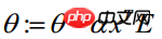
This formula will always be executed iteratively , until convergence is reached ( decreases in each iteration, if the value reduced at a certain step is less than a small value( is less than 0.001), then it is judged to be convergent) or until a certain stopping condition (such as the number of iterations reaches a certain specified value or the algorithm reaches a certain allowable error range).

2, vectorization Vectorization solution

##Vectorization uses matrix calculations instead of for loops to simplify the calculation process ,Improve efficiency. As shown in the above formula, Σ(...) is a summation process, which obviously requires a for statement to loop m times, so vectorization is not fully implemented at all. The vectorization process is introduced below:

The matrix form of the training data is agreed to be as follows. Each row of x is a training sample, and each column has a different special value:

The parameter A of g(A) is a column of vectors, so when implementing the g function Supports column vectors as arguments and returns column vectors. It can be seen from the above formula that hθ(x)-y can be calculated from g(A)-y in one step.

θThe update process can be changed to:

##To sum up, the steps for updating θ after Vectorization are as follows:

(1) Find A=X*θ(this is matrix multiplication, X is a (m, n 1)-dimensional vector, θ is a (n 1, 1)-dimensional column vector, A is a (m, 1)-dimensional vector)

## (2) Find E=g(A)-y (E, y are (m,1)-dimensional column vectors)

(3) Find

(a represents the step size )

3, the choice of step size a

a The value is also a key point to ensure the convergence of gradient descent. If the value is too small, the convergence will be slow, and if the value is too large, the iterative process will not be guaranteed to converge (passing the minimum value). To ensure that the gradient descent algorithm operates correctly, it is necessary to ensure that J(θ) decreases in each iteration. If the value of the step size a is correct, then J(θ) should become smaller and smaller. Therefore, the criterion for judging the value of a is: if J(θ) becomes smaller, it indicates that the value is correct, otherwise, reduce the value of a.

The experience of choosing step size a is: choose a value a, each time about 3 times the previous number. If the iteration cannot proceed normally (J increases, the step size is too large and it crosses the bottom of the bowl) ), consider using a smaller step size. If the convergence is slow, consider increasing the step size. Examples of a values ​​are:

…, 0.001, 0.003, 0.01, 0.03, 0.1 , 0.3, 1….

4, feature value normalization

Logistic regression is also a regression algorithm, multi-dimensional feature training data When using the gradient method to solve regression, the eigenvalues ​​must be scaled to ensure that the value range of the feature is within the same scale before the calculation process converges (because the eigenvalue range may be very different, for example, the value of feature 1 is (1000- 2000), the value of feature 2 is (0.1-0.2)). The method of feature scaling can be customized. Commonly used ones are:

1) mean normalization (or standardization)

(X - mean(X ))/std(X), std(X) represents the standard deviation of the sample

2) rescaling

(X - min) / (max - min)

5, algorithm optimization--stochastic gradient method

Gradient ascent (descent) algorithm The entire data set needs to be traversed every time the regression coefficients are updated. This method is OK when processing about 100 data sets, but if there are billions of samples and thousands of features, the computational complexity of this method will be Too high. An improved method is to update the regression coefficients with only one sample point at a time, which is called the stochastic gradient algorithm. Since the classifier can be incrementally updated when new samples arrive, it can complete parameter updates when new data arrives without the need to re-read the entire data set for batch processing. Therefore, the stochastic gradient algorithm is an online Learning algorithms. (Corresponding to "online learning", processing all data at once is called "batch processing"). The stochastic gradient algorithm is equivalent to the gradient algorithm but is more computationally efficient.

(3) Implementing Logistic Regression Algorithm in Python

The previous section used Andrew Ng’s course to learn about J(θ) =-(1/m)l(θ) is solved using the gradient descent method, which illustrates the solution process of logistic regression. In this section, the process of implementing the algorithm in Python still directly uses the gradient ascent method or the stochastic gradient ascent method to solve J(θ). LRTrain The object also implements the solution process using the gradient ascent method or the stochastic gradient ascent method.

The LR classifier learning package contains three modules: lr.py/object_json.py/test.py. The lr module implements the LR classifier through the object logisticRegres, supporting two solution methods: gradAscent('Grad') and randomGradAscent('randomGrad') (choose one of the two, classifierArray only stores one classification solution result, of course you can also define two classifierArray supports both solution methods).

The test module is an application that uses the LR classifier to predict the mortality of sick horses based on hernia symptoms. There is a problem with this data - the data has a 30% loss rate, which is replaced by the special value 0 because 0 will not affect the weight update of the LR classifier.

The partial missing of sample feature values ​​in the training data is a very thorny problem. Many literatures are devoted to solving this problem, because it is a pity to throw away the data directly and the cost of reacquisition is also expensive. Some optional methods for handling missing data include:

□ Use the mean of available features to fill missing values;

□ Use special values ​​to ±True complement missing values, such as -1;

□ Ignore samples with missing values;

□ Use the mean of similar samples to fill in missing values;

□ Use Additional machine learning algorithms predict missing values.

LR classifier algorithm learning package download address is:

machine learning Logistic regression

(4) Logistic Regression Application

The main purpose of Logistic Regression:

Looking for danger Factors: Looking for risk factors for a certain disease, etc.;

Prediction: According to the model, predict the probability of a certain disease or situation under different independent variables;

Discrimination: In fact, it is somewhat similar to prediction. It is also based on the model to determine the probability that someone belongs to a certain disease or a certain situation, that is, to see how likely this person is. Sex belongs to a certain disease.

Logistic regression is mainly used in epidemiology. A common situation is to explore the risk factors of a certain disease, predict the probability of a certain disease based on the risk factors, etc. For example, if you want to explore the risk factors for gastric cancer, you can choose two groups of people, one is the gastric cancer group, and the other is the non-gastric cancer group. The two groups of people must have different physical signs and lifestyles. The dependent variable here is whether it is gastric cancer, that is, "yes" or "no". The independent variables can include many, such as age, gender, eating habits, Helicobacter pylori infection, etc. The independent variables can be either continuous or categorical.

related suggestion:

Logistic regression ladder descent calculation maximum value

LR in-depth understanding

Brief description of the principles of common machine learning algorithms (LDA, CNN, LR)

LR derivation

The above is the detailed content of Python implements LR classic algorithm. For more information, please follow other related articles on the PHP Chinese website!