


In this tutorial, you will learn what an Excel array formula is, how to enter it correctly in your worksheets, and how to use array constants and array functions.
Array formulas in Excel are an extremely powerful tool and one of the most difficult to master. A single array formula can perform multiple calculations and replace thousands of usual formulas. And still, 90% of users have never used array functions in their worksheets simply because they are scared to start learning them.
Indeed, array formulas one of the most confusing Excel features to learn. The aim of this tutorial is to make the learning curve as easy and smooth as possible.
What is an array in Excel?
Before we start on array functions and formulas, let's figure out what the term "array" means. Essentially, an array is a collection of items. The items can be text or numbers and they can reside in a single row or column, or in multiple rows and columns.
For example, if you put your weekly grocery list into an Excel array format, it would look like:
{"Milk", "Eggs", "Butter", "Corn flakes"}
Then, if you select cells A1 through D1, enter the above array preceded by an equal sign (=) in the formula bar and press CTRL SHIFT ENTER, you will get the following result:

What you have just done is create a one-dimensional horizontal array. Nothing dreadful so far, right?
What is an array formula in Excel?
The difference between an array formula and a regular formula is that an array formula processes several values instead of just one. In other words, an array formula in Excel evaluates all individual values in an array and performs multiple calculations on one or several items according to the conditions expressed in the formula.
Not only can an array formula deal with several values simultaneously, it can also return several values at a time. So, the results returned by an array formula is also an array.
Array formulas are available in all versions of Excel 2019, Excel 2016, Excel 2013, Excel 2010, Excel 2007 and lower.
And now, it seems to be the right time for you to create your first array formula.
Simple example of Excel array formula
Suppose you have some items in column B, their prices in column C, and you want to calculate the grand total of all sales.
Of course, nothing prevents you from calculating subtotals in each row first with something as simple as =B2*C2 and then sum those values:

However, an array formula can spare you those extra key strokes since it gets Excel to store intermediate results in memory rather than in an additional column. So, all it takes is a single array formula and 2 quick steps:
- Select an empty cell and enter the following formula in it:
=SUM(B2:B6*C2:C6) - Press the keyboard shortcut CTRL SHIFT ENTER to complete the array formula.
Once you do this, Microsoft Excel surrounds the formula with {curly braces}, which is a visual indication of an array formula.
What the formula does is multiply the values in each individual row of the specified array (cells B2 through C6), add the sub-totals together, and output the grand total:


This simple example shows how powerful an array formula can be. When working with hundreds and thousands of rows of data, just think how much time you can save by entering one array formula in a single cell.
Why use array formulas in Excel?
Excel array formulas are the handiest tool to perform sophisticated calculations and do complex tasks. A single array formula can replace literally hundreds of usual formulas. Array formulas are very good for tasks such as:
- Sum numbers that meet certain conditions, for example sum N largest or smallest values in a range.
- Sum every other row, or every Nth row or column, as demonstrated in this example.
- Count the number of all or certain characters in a specified range. Here is an array formula that counts all chars, and another one that counts any given characters.
How to enter array formula in Excel (Ctrl Shift Enter)
As you already know, the combination of the 3 keys CTRL SHIFT ENTER is a magic touch that turns a regular formula into an array formula.
When entering an array formula in Excel, there are 4 important things to keep in mind:
- Once you've finished typing the formula and simultaneously pressed the keys CTRL SHIFT ENTER, Excel automatically encloses the formula between {curly braces}. When you select such a cell(s), you can see the braces in the formula bar, which gives you a clue that an array formula is in there.
- Manually typing the braces around a formula won't work. You must press the Ctrl Shift Enter shortcut to complete an array formula.
- Every time you edit an array formula, the braces disappear and you must press Ctrl Shift Enter again to save the changes.
- If you forget to press Ctrl Shift Enter, your formula will behave like a usual formula and process only the first value(s) in the specified array(s).
Because all Excel array formulas require pressing Ctrl Shift Enter, they are sometimes called CSE formulas.
Use the F9 key to evaluate portions of an array formula
When working with array formulas in Excel, you can observe how they calculate and store their items (internal arrays) to display the final result you see in a cell. To do this, select one or several arguments within a function's parentheses, and then press the F9 key. To exit the formula evaluation mode, press the Esc key.
In the above example, to see the sub-totals of all products, you select B2:B6*C2:C6, press F9 and get the following result.

Note. Please pay attention that you must select some part of the formula prior to pressing F9, otherwise the F9 key will simply replace your formula with the calculated value(s).
Single-cell and multi-cell array formulas in Excel
Excel array formula can return a result in a single cell or in multiple cells. An array formula entered in a range of cells is called a multi-cell formula. An array formula residing in a single cell is called a single-cell formula.
There exist a few Excel array functions that are designed to return multi-cell arrays, for example TRANSPOSE, TREND, FREQUENCY, LINEST, etc.
Other functions, such as SUM, AVERAGE, AGGREGATE, MAX, MIN, can calculate array expressions when entered into a single cell by using Ctrl Shift Enter.
The following examples demonstrate how to use a single-cell and multi-cell array formula.
Example 1. A single-cell array formula
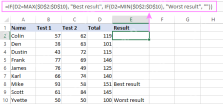
Suppose you have two columns listing the number of items sold in 2 different months, say columns B and C, and you want to find the maximum sales increase.
Normally, you would add an additional column, say column D, that calculates the sales change for each product using a formula like =C2-B2, and then find the maximum value in that additional column =MAX(D:D).
An array formula does not need an additional column since it perfectly stores intermediate results in memory. So, you just enter the following formula and press Ctrl Shift Enter:
=MAX(C2:C6-B2:B6)

Example 2. A multi-cell array formula in Excel
In the previous SUM example, suppose you have to pay 10% tax from each sale and you want to calculate the tax amount for each product with one formula.
Select the range of empty cells, say D2:D6, and enter the following formula in the formula bar:
=B2:B6 * C2:C6 * 0.1
Once you press Ctrl Shift Enter, Excel will place an instance of your array formula in each cell of the selected range, and you will get the following result:

Example 3. Using an Excel array function to return a multi-cell array
As already mentioned, Microsoft Excel provides a few so called "array functions" that are specially designed to work with multi-cell arrays. TRANSPOSE is one of such functions and we are going to utilize it to transpose the above table, i.e. convert rows to columns.
- Select an empty range of cells where you want to output the transposed table. Since we are converting rows to columns, be sure to select the same number of rows and columns as your source table has columns and rows, respectively. In this example, we are selecting 6 columns and 4 rows.
- Press F2 to enter the edit mode.
- Enter the formula and press Ctrl Shift Enter.
In our example, the formula is:
=TRANSPOSE($A$1:$D$6)
The result is going to look similar to this:

This is how you use TRANSPOSE as a CSE array formula in Excel 2019 and earlier. In Dynamic Array Excel, this also works as a regular formula. To learn other ways to transpose in Excel, please check out this tutorial: How to switch columns and rows in Excel.
How to work with multi-cell array formulas
When working with multi-cell array formulas in Excel, be sure to follow these rules to get the correct results:
- Select the range of cells where you want to output the results before entering the formula.
- To delete a multi-cell array formula, either select all the cells containing it and press DELETE, or select the entire formula in the formula bar, press DELETE, and then press Ctrl Shift Enter.
- You cannot edit or move the contents of an individual cell in an array formula, nor can you insert new cells into or delete existing cells from a multi-cell array formula. Whenever you try doing this, Microsoft Excel will throw the warning "You cannot change part of an array".
- To shrink an array formula, i.e. to apply it to fewer cells, you need to delete the existing formula first and then enter a new one.
- To expand an array formula, i.e. apply it to more cells, select all cells containing the current formula plus empty cells where you want to have it, press F2 to switch to the edit mode, adjust the references in the formula and press Ctrl Shift Enter to update it.
- You cannot use multi-cell array formulas in Excel tables.
- You should enter a multi-cell array formula in a range of cells of the same size as the resulting array returned by the formula. If your Excel array formula produces an array larger than the selected range, the excess values won't appear on the worksheet. If an array returned by the formula is smaller than the selected range, #N/A errors will appear in extra cells.
If your formula may return an array with a variable number of elements, enter it in a range equal to or larger than the maximum array returned by the formula and wrap your formula in the IFERROR function, as demonstrated in this example.
Excel array constants
In Microsoft Excel, an array constant is simply a set of static values. These values never change when you copy a formula to other cells or values.
You already saw an example of an array constant created from a grocery list in the very beginning of this tutorial. Now, let's see what other array types exist and how you create them.
There exist 3 types of array constants:
1. Horizontal array constant
A horizontal array constant resides in a row. To create a row array constant, type the values separated by commas and enclose then in braces, for example {1,2,3,4}.
Note. When creating an array constant, you should type the opening and closing braces manually.
To enter a horizontal array in a spreadsheet, select the corresponding number of blank cells in a row, type the formula ={1,2,3,4} in the formula bar, and press Ctrl Shift Enter. The result will be similar to this:

As you see in the screenshot, Excel wraps an array constant in another set of braces, exactly like it does when you are entering an array formula.
2. Vertical array constant
A vertical array constant resides in a column. You create it in the same way as a horizontal array with the only difference that you delimit the items with semicolons, for example:
={11; 22; 33; 44}

3. Two-dimensional array constant
To create a two-dimensional array, you separate each row by a semicolon and each column of data by a comma.
={"a", "b", "c"; 1, 2, 3}

Working with Excel array constants
Array constants are one of the cornerstones of an Excel array formula. The following information and tips might help you use them in the most efficient way.
-
Elements of an array constant
An array constant can contain numbers, text values, Booleans (TRUE and FALSE) and error values, separated by commas or semicolons.
You can enter a numerical value as an integer, decimal, or in scientific notation. If you use text values, they should be surrounded in double quotes (") like in any Excel formula.
An array constant cannot include other arrays, cell references, ranges, dates, defined names, formulas, or functions.
-
Naming array constants
To make an array constant easier to use, give it a name:
- Switch to the Formulas tab > Defined Names group and click Define Name. Alternatively, press Ctrl F3 and click New.
- Type the name in the Name
- In the Refers to box, enter the items of your array constant surrounded in braces with the preceding equality sign (=). For example:
={"Su", "Mo", "Tu", "We", "Th", "Fr", "Sa"} - Click OK to save your named array and close the window.
To enter the named array constant in a sheet, select as many cells in a row or column as there are items in your array, type the array's name in the formula bar preceded with the = sign and press Ctrl Shift Enter.
The result should resemble this:
-
Preventing errors
If your array constant does not work correctly, check for the following problems:
- Delimit the elements of your array constant with the proper character - comma in horizontal array constants and semicolon in vertical ones.
- Selected a range of cells that exactly matches the number of items in your array constant. If you select more cells, each extra cell will have the #N/A error. If you select fewer cells, only a part of the array will be inserted.


Using array constants in Excel formulas
Now that you are familiar with the concept of array constants, let's see how you can use arrays informulas to solve your practical tasks.
Example 1. Sum N largest / smallest numbers in a range
You start by creating a vertical array constant containing as many numbers as you want to sum. For example, if you want to add up 3 smallest or largest numbers in a range, the array constant is {1,2,3}.
Then, you take either LARGE or SMALL function, specify entire range of cells in the first parameter and include the array constant in the second. Finally, embed it in the SUM function, like this:
Sum the largest 3 numbers: =SUM(LARGE(range, {1,2,3}))
Sum the smallest 3 numbers: =SUM(SMALL(range, {1,2,3}))
Don't forget to press Ctrl Shift Enter since you are entering an array formula, and you will get the following result:

In a similar fashion, you can calculate the average of N smallest or largest values in a range:
Average of the top 3 numbers: =AVERAGE(LARGE(range, {1,2,3}))
Average of the bottom 3 numbers: =AVERAGE(SMALL(range, {1,2,3}))
Example 2. Array formula to count cells with multiple conditions
Suppose, you have a list of orders and you want to know how many times a given seller has sold given products.
The easiest way would be using a COUNTIFS formula with multiple conditions. However, if you want to include many products, your COUNTIFS formula may grow too big in size. To make it more compact, you can use COUNTIFS together with SUM and include an array constant in one or several arguments, for example:
=SUM(COUNTIFS(range1, "criteria1", range2, {"criteria1", "criteria2"}))
The real formula may look as follows:
=SUM(COUNTIFS(B2:B9, "sally", C2:C9, {"apples", "lemons"}))

Our sample array consists of only two elements since the goal is to demonstrate the approach. In your real array formulas, you may include as many elements as your business logic requires, provided that the total length of the formula does not exceed 8,192 characters in Excel 2019 - 2007 (1,024 characters in Excel 2003 and lower) and your computer is powerful enough to process large arrays. Please see the limitations of array formulas for more details.
And here is an advanced array formula example that finds the sum of all matching values in a table: SUM and VLOOKUP with an array constant.
AND and OR operators in Excel array formulas
An array operator tells the formula how you want to process the arrays - using AND or OR logic.
- AND operator is the asterisk (*) which is the multiplication symbol. It instructs Excel to return TRUE if ALL of the conditions evaluate to TRUE.
- OR operator is the plus sign ( ). It returns TRUE if ANY of the conditions in a given expression evaluates to TRUE.
Array formula with the AND operator
In this example, we find the sum of sales where the sales person is Mike AND the product is Apples:
=SUM((A2:A9="Mike") * (B2:B9="Apples") * (C2:C9))
Or
=SUM(IF(((A2:A9="Mike") * (B2:B9="Apples")), (C2:C9)))

Technically, this formula multiplies the elements of the three arrays in the same positions. The first two arrays are represented by TRUE and FALSE values which are the results of comparing A2:A9 to Mike" and B2:B9 to "Apples". The third array contains the sales numbers from the range C2:C9. Like any math operation, multiplication converts TRUE and FALSE to 1 and 0, respectively. And because multiplying by 0 always gives zero, the resulting array has 0 when either or both conditions are not met. If both conditions are met, the corresponding element from the third array gets into the final array (e.g. 1*1*C2 = 10). So, the result of multiplication is this array: {10;0;0;30;0;0;0;0}. Finally, the SUM function adds up the array's elements and return a result of 40.
Excel array formula with the OR operator
The following array formula with the OR operator ( ) adds up all sales where the sales person is Mike OR product is Apples:
=SUM(IF(((A2:A9="Mike") (B2:B9="Apples")), (C2:C9)))

In this formula, you add up the elements of the first two arrays (which are the conditions you want to test), and get TRUE (>0) if at least one condition evaluates to TRUE; FALSE (0) when all the conditions evaluates to FALSE. Then, IF checks if the result of addition is greater than 0, and if it is, SUM adds up a corresponding element of the third array (C2:C9).
Tip. In modern versions of Excel, there is no need to use an array formula for this kind of tasks - a simple SUMIFS formula handles them perfectly. Nevertheless, the AND and OR operators in array formulas may prove helpful in more complex scenarios, let alone a very good gymnastics of mind : )
Double unary operator in Excel array formulas
If you've ever worked with array formulas in Excel, chances are you came across a few ones containing a double dash (--) and you may have wondered what it was used for.
A double dash, which is technically called the double unary operator or double negative, is used to convert non-numeric Boolean values (TRUE / FALSE) returned by some expressions into 1 and 0 that an array function can understand.
The following example will hopefully make things easier to understand. Suppose you have a list of dates in column A and you want to know how many dates occur in January, regardless of the year.
The following formula will work a treat:
=SUM(--(MONTH(A2:A10)=1))
Since this is an Excel array formula, remember to press Ctrl Shift Enter to complete it.
If you are interested in some other month, replace 1 with a corresponding number. For example, 2 stands for February, 3 means March, and so on. To make the formula more flexible, you can specify the month number in some cell, like demonstrated in the screenshot:

And now, let's analyze how this array formula works. The MONTH function returns the month of each date in cells A2 through A10 represented by a serial number, which producing the array {2;1;4;2;12;1;2;12;1}.
After that, each element of the array is compared to the value in cell D1, which is number 1 in this example. The result of this comparison is an array of Boolean values TRUE and FALSE. As you remember, you can select a certain portion of an array formula and press F9 to see what that part equates to:

Finally, you have to convert these Boolean values to 1's and 0's that the SUM function can understand. And this is what the double negative sign is needed for. The first unary coerces TRUE/FALSE to -1/0, respectively. The second one negates the values, i.e. reverses the sign, turning them into 1 and 0, which most of Excel functions can understand and work with. If you remove the double unary from the above formula, it won't work.
I am hopeful this short tutorial has proved helpful on your road to mastering Excel array formulas. Next week, we are going to continue with Excel arrays by focusing on advanced formula examples. Please stay tuned and thank you for reading!
The above is the detailed content of Array formulas and functions in Excel - examples and guidelines. For more information, please follow other related articles on the PHP Chinese website!

 How You Can Use Wildcards in Microsoft Excel to Refine Your SearchMay 13, 2025 am 01:59 AM
Excel wildcards: a powerful tool for efficient search and filtering This article will dive into the power of wildcards in Microsoft Excel, including their application in search, formulas, and filters, and some details to note. Wildcards allow you to perform fuzzy matching, making it more flexible to find and process data. *Wildcards: asterisks () and question marks (?)** Excel mainly uses two wildcards: asterisk (*) and question mark (?). *Asterisk (): Any number of characters** The asterisk represents any number of characters, including zero characters. For example: *OK* Match the cell containing "OK", "OK&q
 Excel IF function with multiple conditionsMay 12, 2025 am 11:02 AM
The tutorial shows how to create multiple IF statements in Excel with AND as well as OR logic. Also, you will learn how to use IF together with other Excel functions. In the first part of our Excel IF tutorial, we looked at how to constru
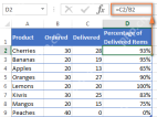 How to calculate percentage in Excel - formula examplesMay 12, 2025 am 10:28 AM
In this tutorial, you will lean a quick way to calculate percentages in Excel, find the basic percentage formula and a few more formulas for calculating percentage increase, percent of total and more. Calculating percentage is useful in m
 Logical operators in Excel: equal to, not equal to, greater than, less thanMay 12, 2025 am 09:41 AM
Logical operators in Excel: The key to efficient data analysis In Excel, many tasks involve comparing data in different cells. To this end, Microsoft Excel provides six logical operators, also known as comparison operators. This tutorial is designed to help you understand the connotation of Excel logical operators and write the most efficient formulas for data analysis. Excel logical operators equal Not equal to Greater than/less than/greater than/six equal to/less than equal to Common uses of logical operators in Excel Overview of Excel Logical Operators Logical operators in Excel are used to compare two values. Logical operators are sometimes called boolean operators because in any given case, the result of comparison
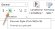 How to show percentage in ExcelMay 12, 2025 am 09:40 AM
This concise guide explores Excel's percentage formatting capabilities, covering various scenarios and advanced techniques. Learn how to format existing values, handle empty cells, and customize your percentage display. To quickly apply percentage f
 Logical functions in Excel: AND, OR, XOR and NOTMay 12, 2025 am 09:39 AM
The tutorial explains the essence of Excel logical functions AND, OR, XOR and NOT and provides formula examples that demonstrate their common and inventive uses. Last week we tapped into the insight of Excel logical operators that are us
 Comments vs. Notes in Microsoft Excel: What's the Difference?May 12, 2025 am 06:03 AM
This guide explores Microsoft Excel's comment and note features, explaining their uses and differences. Both tools annotate cells, but serve distinct purposes and display differently in printed worksheets. Excel Comments: Collaborative Annotations E
 Excel templates: how to make and useMay 11, 2025 am 10:43 AM
Excel template: a tool for efficient office work Microsoft Excel templates are a powerful tool to improve the efficiency of Excel, saving significantly time. After creating a template, you only need a small amount of adjustment to adapt to different scenarios and achieve reuse. Well-designed Excel templates can also improve the aesthetics and consistency of documents, leaving a good impression on colleagues and bosses. The value of templates is particularly prominent for common document types such as calendars, budget planners, invoices, inventory tables, and dashboards. What else is more convenient than just using a spreadsheet that looks beautiful, has a full-featured and is easy to customize? A Microsoft Excel template is a pre-designed workbook or worksheet, most of which


Hot AI Tools

Undresser.AI Undress
AI-powered app for creating realistic nude photos

AI Clothes Remover
Online AI tool for removing clothes from photos.

Undress AI Tool
Undress images for free

Clothoff.io
AI clothes remover

Video Face Swap
Swap faces in any video effortlessly with our completely free AI face swap tool!

Hot Article
Hot Tools

Dreamweaver Mac version
Visual web development tools

SublimeText3 Mac version
God-level code editing software (SublimeText3)

EditPlus Chinese cracked version
Small size, syntax highlighting, does not support code prompt function

MinGW - Minimalist GNU for Windows
This project is in the process of being migrated to osdn.net/projects/mingw, you can continue to follow us there. MinGW: A native Windows port of the GNU Compiler Collection (GCC), freely distributable import libraries and header files for building native Windows applications; includes extensions to the MSVC runtime to support C99 functionality. All MinGW software can run on 64-bit Windows platforms.

SecLists
SecLists is the ultimate security tester's companion. It is a collection of various types of lists that are frequently used during security assessments, all in one place. SecLists helps make security testing more efficient and productive by conveniently providing all the lists a security tester might need. List types include usernames, passwords, URLs, fuzzing payloads, sensitive data patterns, web shells, and more. The tester can simply pull this repository onto a new test machine and he will have access to every type of list he needs.

