


The tutorial shows how to use the SUMIF function in Google spreadsheets to conditionally sum cells. You will find formula examples for text, numbers and dates and learn how to sum with multiple criteria.
Some of the best functions in Google Sheets are those that help you summarize and categorize data. Today, we are going to have a closer look at one of such functions - SUMIF - a powerful instrument to conditionally sum cells. Before studying the syntax and formula examples, let me begin with a couple of important remarks.
Google Sheets has two functions to add up numbers based on conditions: SUMIF and SUMIFS. The former evaluates just one condition while the latter can test multiple conditions at a time. In this tutorial, we will focus solely on the SUMIF function, the use of SUMIFS will be covered in the next article.
If you know how to use SUMIF in Excel desktop or Excel online, SUMIF in Google Sheets will be a piece of cake for you since both are essentially the same. But don't rush to close this page yet - you may find a few unobvious but very useful SUMIF formulas you didn't know!
See the colors, sum the numbers!
Sum up cells by their fill color — effortlessly and accurately

Duplicates? Merge, Sum, Done!
Spot duplicates, combine details, and tally totals

Unlock the full potential of your Google Sheets
Discover your data's sidekick — trusted by millions!

SUMIF in Google Sheets - syntax and basic uses
The SUMIF function is Google Sheets is designed to sum numeric data based on one condition. Its syntax is as follows:
SUMIF(range, criterion, [sum_range])Where:
- Range (required) - the range of cells that should be evaluated by criterion.
- Criterion (required) - the condition to be met.
- Sum_range (optional) - the range in which to sum numbers. If omitted, then range is summed.
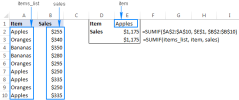
As an example, let's make a simple formula that will sum numbers in column B if column A contains an item equal to the "sample item".
For this, we define the following arguments:
- Range - a list of items - A2:A12.
- Criterion - a cell containing the item of interest - E1.
- Sum_range - amounts to be summed - B2:B12.
Putting all the arguments together, we get the following formula:
=SUMIF(A2:A12,E1,B2:B12)
And it works exactly as it should:

Google Sheets SUMIF examples
From the above example, you may have the impression that using SUMIF formulas in Google spreadsheets is so easy that you could do it with your eyes shut. In most cases, it is really so :) But still there are some tricks and non-trivial uses that could make your formulas more effective. The below examples demonstrate a few typical use cases. To make the examples easier to follow, I invite you to open our sample SUMIF Google Sheet.
SUMIF formulas with text criteria (exact match)
To add up numbers that have a specific text in another column in the same row, your simply supply the text of interest in the criterion argument of your SUMIF formula. As usual, any text in any argument of any formula should be enclosed in "double quotes".
For example, to get a total of bananas, you use this formula:
=SUMIF(A5:A15,"bananas",B5:B15)
Or, you can put the criterion in some cell and refer to that cell:
=SUMIF(A5:A15,B1,B5:B15)
This formula is crystal clear, isn't it? Now, how do you get a total of all items except bananas? For this, use the not equal to operator:
=SUMIF(A5:A15,"bananas",B5:B15)
If an "exclusion item" is input in a cell, then you enclose the not equal to operator in double quotes ("") and concatenate the operator and cell reference by using an ampersand (&). For example:
=SUMIF (A5:A15,""&B1, B5:B15)
The following screenshot demonstrates both "Sum if equal to" and "Sum if not equal to" formulas in action:

Please note that SUMIF in Google Sheets searches for the specified text exactly. In this example, only Bananas amounts are summed, Green bananas and Goldfinger bananas are not included. To sum with partial match, use wildcard characters as shown in the next example.
SUMIF formulas with wildcard characters (partial match)
In situations when you want to sum cells in one column if a cell in another column contains a specific text or character as part of the cell contents, include one of the following wildcards in your criteria:
- Question mark (?) to match any single character.
- Asterisk (*) to match any sequence of characters.
For example, to sum the amounts of all sorts of bananas, use this formula:
=SUMIF(A2:A13,"*bananas*",B2:B13)
You can also use wildcards together with cell references. For this, enclose the wildcard character in quotation marks, and concatenate it with a cell reference:
=SUMIF(A2:A13, "*"&E1&"*", B2:B13)
Either way, our SUMIF formula adds up the amounts of all bananas:

To match an actual question mark or asterisk, prefix it with the tilde (~) character like "~?" or "~*".
For example, to sum numbers in column B that have an asterisk in column A in the same row, use this formula:
=SUMIF(A2:A13, "~*", B2:B13)
You can even type an asterisk in some cell, say B1, and concatenate that cell with the tilde char:
=SUMIF(A2:A13, "~"&E1, B2:B13)

Case-sensitive SUMIF in Google Sheets
By default, SUMIF in Google Sheets does not see the difference between small and capital letters. For force it to teat uppercase and lowercase characters differently, use SUMIF in combination with the FIND and ARRAYFORMULA functions:
SUMIF(ARRAYFORMULA( FIND("text", range)), 1, sum_range)Supposing you have a list of order numbers in A2:A12 and corresponding amounts in C2:C12, where the same order number appears in several rows. You enter the target order id in some cell, say F1, and use the following formula to return the order total:
=SUMIF(ARRAYFORMULA(FIND(F1, A2:A12)),1, C2:C12)

How this formula works
To better understand the formula's logic, let's break it down into the meaningful parts:
The trickiest part is the range argument: ARRAYFORMULA(FIND(F1, A2:A12))
You use the case-sensitive FIND function to look for the exact order id. The problem is that a regular FIND formula can only search within a single cell. To search within a range, an array formula is needed, so you nest FIND inside ARRAYFORMULA.
When the above combination finds an exact match, it returns 1 (the position of the first found character), otherwise a #VALUE error. So, the only thing left for you to do is to sum the amounts corresponding to 1's. For this, you put 1 in the criterion argument, and C2:C12 in the sum_range argument. Done!
SUMIF formulas for numbers
To sum numbers that meet a certain condition, use one of the comparison operators in your SUMIF formula. In most cases, choosing an appropriate operator is not a problem. Embedding it in the criterion properly could be a challenge.
Sum if greater than or less than
To compare the source numbers to a particular number, use one of the following logical operators:
- greater than (>)
- less than (
- greater than or equal to (>=)
- less than or equal to (
For example, to add up numbers in B2:B12 that are greater than 200, use this formula:
=SUMIF(B2:B12, ">200", B2:B12)
Please notice the correct syntax of the criterion: a number prefixed with a comparison operator, and the whole construction enclosed in quotation marks.

Or, you can type the number in some cell, and concatenate the comparison operator with a cell reference:
=SUMIF(B2:B12, ">"&E1, B2:B12)

You can even input both the comparison operator and number in separate cells, and concatenate those cells:
=SUMIF(B2:B12, E1&F1)

In a similar manner, you can use other logical operators such as:
Sum if greater than or equal to 200:
=SUMIF(B2:B12, ">=200")
Sum if less than 200:
=SUMIF(B2:B12, "
Sum if less than or equal to 200:
To sum numbers that equal a specific number, you can use the equality sign (=) together with the number or omit the equality sign and include only the number in the criterion argument. For example, to add up amounts in column B whose quantity in column C is equal to 10, use any of the below formulas: or or Where F1 is the cell with the required quantity.
To sum numbers other than the specified number, use the not equal to operator (). In our example, to add up the amounts in column B that have any quantity except 10 in column C, go with one of these formulas: The screenshot below shows the result:
To conditionally sum values based on date criteria, you also use the comparison operators like shown in the above examples. The key point is that a date should be supplied in the format that Google Sheets can understand. For instance, to sum amounts in B2:B12 for delivery dates prior to 11-Apr-2024, build the criterion in one of these ways: Where F1 is the target date:
In case you want to conditionally sum cells based on today's date, include the TODAY() function in the criterion argument. As an example, let's make a formula that adds up the amounts for today's deliveries: Taking the example further, we can find a total of past and future deliveries: Before today: After today: In many situations, you may need to sum values in a certain column if a corresponding cell in another column is or is not empty. For this, use one of the following criteria in your Google Sheets SUMIF formulas: For example, to sum the amounts for which the delivery date is set (a cell in column C is not empty), use this formula: To get a total of the amounts with no delivery date (a cell in column C is empty), use this one: The SUMIF function in Google Sheets is designed to add up values based on just one criterion. To sum with multiple criteria, you can add two or more SUMIF functions together. For example, to sum Apples and Oranges amounts, utilize this formula: Or, put the item names in two separate cells, say E1 and E2, and use each of those cells as a criterion: Please note that this formula works like SUMIF with OR logical - it sums values if at least one of the specified criteria is met. In this example, we add values in column B if column A equals "apples" or "oranges". In other words, SUMIF() SUMIF() works like the following pseudo-formula (not a real one, it only demonstrates the logic!): sumif(A:A, "apples" or "oranges", B:B). If you are looking to conditionally sum with AND logical, i.e. add up values when all of the specified criteria are met, use the Google Sheets SUMIFS function.
Now that you know the nuts and bolts of the SUMIF function in Google Sheets, it may be a good idea to make a short summary of what you've already learned. The syntax of the SUMIF function allows for only one range, one criterion and one sum_range. To sum with multiple criteria, either add several SUMIF functions together (OR logic) or use SUMIFS formulas (AND logic).
If you are looking for a case-sensitive SUMIF formula that can differentiate between uppercase and lowercase characters, use SUMIF in combination with ARRAYFORMULA and FIND as shown in this example.
In fact, the sum_range argument specifies only the upper leftmost cell of the range to sum, the remaining area is defined by the dimensions of the range argument. To put it differently, SUMIF(A1:A10, "apples", B1:B10) and SUMIF(A1:A10, "apples", B1:B100) will both sum values in the range B1:B10 because it is the same size as range (A1:A10). So, even if you mistakenly supply a wrong sum range, Google Sheets will still calculate your formula right, provided the top left cell of sum_range is correct. That said, it is still recommended to provide equally sized range and sum_range to avoid mistakes and prevent inconsistency issues.
For your Google Sheets SUMIF formula to work correctly, express the criteria the right way: If you plan to copy or move your SUMIF formula at a later point, fix the ranges by using absolute cell references (with the $ sign) like in SUMIF($A$2:$A$10, "apples", $B$2:$B$10). This is how you use the SUMIF function in Google Sheets. To have a closer look at the formulas discussed in this tutorial, you are welcome to open our sample SUMIF Google Sheet. I thank you for reading and hope to see you on our blog next week!
Sample SUMIF Spreadsheet=SUMIF(B2:B12, "
Sum if equal to
=SUMIF(C2:C12, 10, B2:B12)=SUMIF(C2:C12, "=10", B2:B12)=SUMIF(C2:C12, F1, B2:B12) 
Sum if not equal to
=SUMIF(C2:C12, "10", B2:B12)=SUMIF(C2:C12, ""&F1, B2:B12)
Google Sheets SUMIF formulas for dates
=SUMIF(C2:C12, "=SUMIF(C2:C12, "=SUMIF(C2:C12, "
=SUMIF(C2:C12, TODAY(), B2:B12)

=SUMIF(C2:C12, "=SUMIF(C2:C12, ">"&TODAY(), B2:B12)
Sum based on blank or non-blank cells
Sum if blank:
Sum if not blank:
=SUMIF(C5:C15, "", B5:B15)=SUMIF(C5:C15, "", B5:B15)

Google Sheets SUMIF with multiple criteria (OR logic)
=SUMIF(A2:A12, "apples", B2:B12) SUMIF(A2:A12, "oranges", B2:B12)=SUMIF(A2:A12, E1, B2:B12) SUMIF(A2:A12, E2, B2:B12)

Google Sheets SUMIF - things to remember
1. SUMIF can evaluate only one condition
2. The SUMIF function is case-insensitive
3. Supply equally sized range and sum_range
4. Mind the syntax of SUMIF criteria
=SUMIF(A2:A10, "apples", B2:B10) =SUMIF(A2:A10, "*", B2:B10) =SUMIF(A2:A10, ">5")=SUMIF(A5:A10, "apples", B5:B10)=SUMIF(A2:A10, ">"&B2) =SUMIF(A2:A10, ">"&TODAY(), B2:B10)5. Lock ranges with absolute cell references if needed
Spreadsheet with formula examples
The above is the detailed content of SUMIF in Google Sheets with formula examples. For more information, please follow other related articles on the PHP Chinese website!

 MEDIAN formula in Excel - practical examplesApr 11, 2025 pm 12:08 PM
This tutorial explains how to calculate the median of numerical data in Excel using the MEDIAN function. The median, a key measure of central tendency, identifies the middle value in a dataset, offering a more robust representation of central tenden
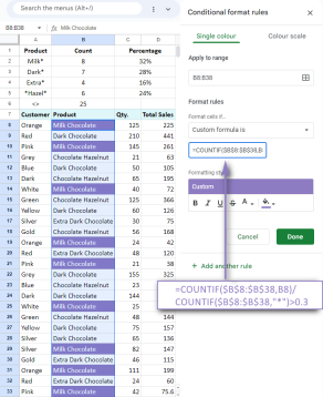 Google Spreadsheet COUNTIF function with formula examplesApr 11, 2025 pm 12:03 PM
Master Google Sheets COUNTIF: A Comprehensive Guide This guide explores the versatile COUNTIF function in Google Sheets, demonstrating its applications beyond simple cell counting. We'll cover various scenarios, from exact and partial matches to han
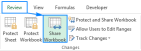 Excel shared workbook: How to share Excel file for multiple usersApr 11, 2025 am 11:58 AM
This tutorial provides a comprehensive guide to sharing Excel workbooks, covering various methods, access control, and conflict resolution. Modern Excel versions (2010, 2013, 2016, and later) simplify collaborative editing, eliminating the need to m
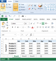 How to convert Excel to JPG - save .xls or .xlsx as image fileApr 11, 2025 am 11:31 AM
This tutorial explores various methods for converting .xls files to .jpg images, encompassing both built-in Windows tools and free online converters. Need to create a presentation, share spreadsheet data securely, or design a document? Converting yo
 Excel names and named ranges: how to define and use in formulasApr 11, 2025 am 11:13 AM
This tutorial clarifies the function of Excel names and demonstrates how to define names for cells, ranges, constants, or formulas. It also covers editing, filtering, and deleting defined names. Excel names, while incredibly useful, are often overlo
 Standard deviation Excel: functions and formula examplesApr 11, 2025 am 11:01 AM
This tutorial clarifies the distinction between standard deviation and standard error of the mean, guiding you on the optimal Excel functions for standard deviation calculations. In descriptive statistics, the mean and standard deviation are intrinsi
 Square root in Excel: SQRT function and other waysApr 11, 2025 am 10:34 AM
This Excel tutorial demonstrates how to calculate square roots and nth roots. Finding the square root is a common mathematical operation, and Excel offers several methods. Methods for Calculating Square Roots in Excel: Using the SQRT Function: The
 Google Sheets basics: Learn how to work with Google SpreadsheetsApr 11, 2025 am 10:23 AM
Unlock the Power of Google Sheets: A Beginner's Guide This tutorial introduces the fundamentals of Google Sheets, a powerful and versatile alternative to MS Excel. Learn how to effortlessly manage spreadsheets, leverage key features, and collaborate


Hot AI Tools

Undresser.AI Undress
AI-powered app for creating realistic nude photos

AI Clothes Remover
Online AI tool for removing clothes from photos.

Undress AI Tool
Undress images for free

Clothoff.io
AI clothes remover

AI Hentai Generator
Generate AI Hentai for free.

Hot Article
Hot Tools

Safe Exam Browser
Safe Exam Browser is a secure browser environment for taking online exams securely. This software turns any computer into a secure workstation. It controls access to any utility and prevents students from using unauthorized resources.

MinGW - Minimalist GNU for Windows
This project is in the process of being migrated to osdn.net/projects/mingw, you can continue to follow us there. MinGW: A native Windows port of the GNU Compiler Collection (GCC), freely distributable import libraries and header files for building native Windows applications; includes extensions to the MSVC runtime to support C99 functionality. All MinGW software can run on 64-bit Windows platforms.

SecLists
SecLists is the ultimate security tester's companion. It is a collection of various types of lists that are frequently used during security assessments, all in one place. SecLists helps make security testing more efficient and productive by conveniently providing all the lists a security tester might need. List types include usernames, passwords, URLs, fuzzing payloads, sensitive data patterns, web shells, and more. The tester can simply pull this repository onto a new test machine and he will have access to every type of list he needs.

WebStorm Mac version
Useful JavaScript development tools

Dreamweaver CS6
Visual web development tools

