


DATEDIF and NETWORKDAYS in Google Sheets: date difference in days, months and years

Today's blog post is all about figuring out the difference between two dates in Google Sheets. You will see lots of DATEDIF formulas to count days, months and years, and learn how NETWORKDAYS is used to count workdays only even if your holidays are based on a custom schedule.
Lots of spreadsheets users find dates confusing, if not extremely difficult, to handle. But believe it or not, there are a few handy and straightforward functions for that purpose. DATEDIF and NETWORKDAYS are a couple of them.
DATEDIF function in Google Sheets
As it happens with functions, their names suggest the action. The same goes for DATEDIF. It must be read as date dif, not dated if, and it stands for date difference. Hence, DATEDIF in Google Sheets calculates the date difference between two dates.
Let's break it down to pieces. The function requires three arguments:
=DATEDIF(start_date, end_date, unit)-
start_date – a date used as a starting point. It must be one of the following:
- a date itself in double-quotes: "8/13/2020"
- a reference to a cell with a date: A2
- a formula that returns a date: DATE(2020, 8, 13)
- a number that stands for a particular date and that can be interpreted as a date by Google Sheets, e.g. 44056 represents August 13, 2020.
- end_date – a date used as an endpoint. It must be of the same format as the start_date.
-
unit – is used to tell the function what difference to return. Here's a full list of units you can use:
- "D" – (short for days) returns the number of days between two dates.
- "M" – (months) the number of full months between two dates.
- "Y" – (years) the number of full years.
- "MD" – (days ignoring months) the number of days after subtracting whole months.
- "YD" – (days ignoring years) the number of days after subtracting whole years.
- "YM" – (months ignoring years) the number of complete months after subtracting full years.
Note. All units must be put to formulas the same way they appear above – in double-quotes.
Now let's piece all these parts together and see how DATEDIF formulas work in Google Sheets.
Calculate days between two dates in Google Sheets
Example 1. Count all days
I have a small table to track some orders. All of them have been shipped in the first half of August – Shipping date – which is going to be my start date. There's also an approximate delivery date – Due date.

I'm going to calculate days – "D" – between shipping and due dates to see how long it takes for items to arrive. Here is the formula I should use:
=DATEDIF(B2, C2, "D")

I enter the DATEDIF formula to D2 and then copy it down the column to apply to other rows.
Tip. You can always calculate the entire column at once with a single formula using ARRAYFORMULA:
=ArrayFormula(DATEDIF(B2:B13, C2:C13, "D"))

Example 2. Count days ignoring months
Imagine there are a few months between two dates:

How do you count only days as if they belonged to the same month? That's right: by ignoring full months that have passed. DATEDIF calculates this automatically when you use the "MD" unit:
=DATEDIF(A2, B2, "MD")

The function subtracts elapsed months and counts remaining days.
Example 3. Count days ignoring years
Another unit – "YD" – will aid for when dates have more than a year between them:
=DATEDIF(A2, B2, "YD")

The formula will subtract years first, and then calculate remaining days as if they belonged to the same year.
Count working days in Google Sheets
There is a special case when you need to count only working days in Google Sheets. DATEDIF formulas won't be much of a help here. And I believe you will agree that subtracting weekends manually is not the most elegant option.
Luckily, Google Sheets has a couple of not-so-magic spells for that :)
Example 1. NETWORKDAYS function
The first one is called NETWORKDAYS. This function calculates the number of working days between two dates excluding weekends (Saturday and Sunday) and even holidays if necessary:
=NETWORKDAYS(start_date, end_date, [holidays])-
start_date – a date used as a starting point. Required.
Note. If this date is not a holiday, it is counted as a working day.
-
end_date – a date used as an endpoint. Required.
Note. If this date is not a holiday, it is counted as a working day.
- holidays – this one is optional for when you need to point out specific holidays. It must be a range of dates or numbers representing dates.
To illustrate how it works, I will add a list of holidays that take place in-between shipping and due dates:

So, column B is my start date, columns C – end date. Dates in column E are the holidays to consider. Here is how the formula should look:
=NETWORKDAYS(B2, C2, $E$2:$E$4)

Tip. If you're going to copy the formula to other cells, use absolute cells references for holidays to avoid errors or incorrect results. Or consider building an array formula instead.
Have you noticed how the number of days decreased compared to the DATEDIF formulas? Because now the function automatically subtracts all Saturdays, Sundays, and two holidays that take place on Friday and Monday.
Note. Unlike DATEDIF in Google Sheets, NETWORKDAYS counts start_day and end_day as workdays unless they are holidays. Hence, D7 returns 1.
Example 2. NETWORKDAYS.INTL for Google Sheets
If you have a custom weekend schedule, you will benefit from another function: NETWORKDAYS.INTL. It lets you count working days in Google Sheets based on personally set weekends:
=NETWORKDAYS.INTL(start_date, end_date, [weekend], [holidays])- start_date – a date used as a starting point. Required.
-
end_date – a date used as an endpoint. Required.
Note. NETWORKDAYS.INTL in Google Sheets also counts start_day and end_day as workdays unless they are holidays.
-
weekend – this one is optional. If omitted, Saturday and Sunday are considered to be weekends. But you can alter that using two ways:
-
Masks.
Tip. This way is perfect for when your days off are scattered all over the week.
Mask is a seven-digit pattern of 1's and 0's. 1 stands for a weekend, 0 for a workday. The first digit in the pattern is always Monday, the last one – Sunday.
For example, "1100110" means that you work on Wednesday, Thursday, Friday, and Saturday.
Note. The mask must be put in double-quotes.
-
Numbers.
Use one-digit numbers (1-7) that denote a pair of set weekends:
Number Weekend 1 Saturday, Sunday 2 Sunday, Monday 3 Monday, Tuesday 4 Tuesday, Wednesday 5 Wednesday, Thursday 6 Thursday, Friday 7 Friday, Saturday Or work with two-digit numbers (11-17) that denote one day to rest within a week:
Number Weekend day 11 Sunday 12 Monday 13 Tuesday 14 Wednesday 15 Thursday 16 Friday 17 Saturday
-
Masks.
- holidays – it is also optional and is used to specify holidays.
This function may seem complicated because of all those numbers, but I encourage you to give it a try.
First, just get a clear understanding of your days off. Let's make it Sunday and Monday. Then, decide on the way to indicate your weekends.
If you go with a mask, it will be like this – 1000001:
=NETWORKDAYS.INTL(B2, C2, "1000001")
But since I have two weekend days in a row, I can use a number from the tables above, 2 in my case:
=NETWORKDAYS.INTL(B2, C2, 2)
Then simply add the last argument – refer to holidays in column E, and the formula is ready:
=NETWORKDAYS.INTL(B2, C2, 2, $E$2:$E$4)

Google Sheets and date difference in months
Sometimes months matter more than days. If this is true for you and you prefer getting the date difference in months rather than days, let Google Sheets DATEDIF do the job.
Example 1. The number of full months between two dates
The drill is the same: the start_date goes first, followed by the end_date and "M" – that stands for months – as a final argument:
=DATEDIF(A2, B2, "M")

Tip. Don't forget about the ARRAUFORMULA function that can help you count months on all rows at once:
=ARRAYFORMULA(DATEDIF(A2:A13, B2:B13, "M"))
Example 2. The number of months ignoring years
You may not need to count months throughout all years in-between start and end dates. And DATEDIF lets you do that.
Just use the "YM" unit and the formula will subtract whole years first, and then count the number of months between dates:
=DATEDIF(A2, B2, "YM")

Calculate years between two dates in Google Sheets
The last (but not least) thing to show you is how Google Sheets DATEDIF calculates the date difference in years.
I'm going to calculate the number of years couples have been married based on their wedding dates and today's date:

As you may have already guessed, I will use the "Y" unit for that:
=DATEDIF(A2, B2, "Y")

All these DATEDIF formulas are the first to try when it comes to calculating days, months, and years between two dates in Google Sheets.
If your case can't be solved by these or if you have any questions, I encourage you to share them with us in the comments section below.
The above is the detailed content of DATEDIF and NETWORKDAYS in Google Sheets: date difference in days, months and years. For more information, please follow other related articles on the PHP Chinese website!

 MEDIAN formula in Excel - practical examplesApr 11, 2025 pm 12:08 PM
This tutorial explains how to calculate the median of numerical data in Excel using the MEDIAN function. The median, a key measure of central tendency, identifies the middle value in a dataset, offering a more robust representation of central tenden
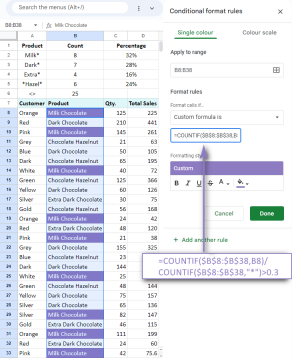 Google Spreadsheet COUNTIF function with formula examplesApr 11, 2025 pm 12:03 PM
Master Google Sheets COUNTIF: A Comprehensive Guide This guide explores the versatile COUNTIF function in Google Sheets, demonstrating its applications beyond simple cell counting. We'll cover various scenarios, from exact and partial matches to han
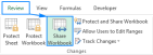 Excel shared workbook: How to share Excel file for multiple usersApr 11, 2025 am 11:58 AM
This tutorial provides a comprehensive guide to sharing Excel workbooks, covering various methods, access control, and conflict resolution. Modern Excel versions (2010, 2013, 2016, and later) simplify collaborative editing, eliminating the need to m
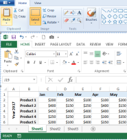 How to convert Excel to JPG - save .xls or .xlsx as image fileApr 11, 2025 am 11:31 AM
This tutorial explores various methods for converting .xls files to .jpg images, encompassing both built-in Windows tools and free online converters. Need to create a presentation, share spreadsheet data securely, or design a document? Converting yo
 Excel names and named ranges: how to define and use in formulasApr 11, 2025 am 11:13 AM
This tutorial clarifies the function of Excel names and demonstrates how to define names for cells, ranges, constants, or formulas. It also covers editing, filtering, and deleting defined names. Excel names, while incredibly useful, are often overlo
 Standard deviation Excel: functions and formula examplesApr 11, 2025 am 11:01 AM
This tutorial clarifies the distinction between standard deviation and standard error of the mean, guiding you on the optimal Excel functions for standard deviation calculations. In descriptive statistics, the mean and standard deviation are intrinsi
 Square root in Excel: SQRT function and other waysApr 11, 2025 am 10:34 AM
This Excel tutorial demonstrates how to calculate square roots and nth roots. Finding the square root is a common mathematical operation, and Excel offers several methods. Methods for Calculating Square Roots in Excel: Using the SQRT Function: The
 Google Sheets basics: Learn how to work with Google SpreadsheetsApr 11, 2025 am 10:23 AM
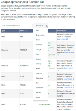
Unlock the Power of Google Sheets: A Beginner's Guide This tutorial introduces the fundamentals of Google Sheets, a powerful and versatile alternative to MS Excel. Learn how to effortlessly manage spreadsheets, leverage key features, and collaborate


Hot AI Tools

Undresser.AI Undress
AI-powered app for creating realistic nude photos

AI Clothes Remover
Online AI tool for removing clothes from photos.

Undress AI Tool
Undress images for free

Clothoff.io
AI clothes remover

Video Face Swap
Swap faces in any video effortlessly with our completely free AI face swap tool!

Hot Article
Hot Tools

Notepad++7.3.1
Easy-to-use and free code editor

DVWA
Damn Vulnerable Web App (DVWA) is a PHP/MySQL web application that is very vulnerable. Its main goals are to be an aid for security professionals to test their skills and tools in a legal environment, to help web developers better understand the process of securing web applications, and to help teachers/students teach/learn in a classroom environment Web application security. The goal of DVWA is to practice some of the most common web vulnerabilities through a simple and straightforward interface, with varying degrees of difficulty. Please note that this software

WebStorm Mac version
Useful JavaScript development tools

SublimeText3 English version
Recommended: Win version, supports code prompts!

SublimeText3 Mac version
God-level code editing software (SublimeText3)

