


Excel 365's revolutionary computing engine update makes array formulas easy to understand, no longer just a dedicated skill for advanced users. This tutorial explains the concept of Excel dynamic arrays and shows how to use them to improve worksheet efficiency and simplify settings.
Excel array formulas have always been considered the patent of experts and formula experts. The sentence "can be solved with array formulas" often causes many users to immediately respond: "Is there any other way?"
The introduction of dynamic arrays is a long-awaited and very welcome change. Because they are able to handle multiple values in a simple way, without any tricks and tricks, every Excel user can understand and easily create dynamic array formulas.
- Dynamic array availability
- Dynamic array functions
- Example of dynamic array formulas
- Overflow area - one formula, multiple cells
- Overflow area reference (# symbol)
- Implicit intersection and @ characters
- Advantages of dynamic arrays
- Limitations of dynamic arrays
- Dynamic arrays and traditional CSE array formulas
- Backward compatibility
- Excel dynamic array formula is invalid
Excel dynamic array
Dynamic arrays are resized arrays that automatically calculate and return values to multiple cells, all based on formulas entered in a single cell.
Microsoft Excel has undergone many changes over the past thirty years, but one thing is consistent: a formula, a cell. Even with traditional array formulas, you need to enter the formula in each cell where you want to display the result. With dynamic arrays, this rule no longer applies. Now any formula that returns the array value will automatically overflow into adjacent cells without pressing Ctrl Shift Enter or doing anything else. In other words, manipulating a dynamic array is as simple as manipulating a single cell.
Let's use a very basic example to illustrate this concept. Suppose you need to multiply two sets of numbers, for example, calculate different percentages.
In the non-dynamic version of Excel, the following formula only applies to the first cell unless you enter it in multiple cells and press Ctrl Shift Enter to explicitly set it as an array formula:
=A3:A5*B2:D2

Now, see what happens when using the same formula in Excel 365. You simply enter it in a cell (B3 in this case), press Enter... the entire area will immediately fill in the result:

Filling multiple cells with a single formula is called overflow , and the filled area of cells is called overflow.
It should be noted that recent updates are more than just a new way to deal with Excel arrays. In fact, this is a breakthrough change to the entire computing engine. With dynamic arrays, a series of new functions have been added to the Excel function library, and existing functions have also started to run faster and more efficiently. Ultimately, the new dynamic array should completely replace the old-style array formulas entered using the Ctrl Shift Enter shortcut.
Excel Dynamic Array Availability
Dynamic arrays were launched at the Microsoft Ignite conference in 2018 and were released to Office 365 subscribers in January 2020. Currently, they are available in Microsoft 365 subscriptions and Excel 2021.
The following versions support dynamic arrays:
- Excel 365 for Windows
- Excel 365 for Mac
- Excel 2021
- Excel 2021 for Mac
- Excel for iPad
- Excel for iPhone
- Android Tablet Version Excel
- Android mobile version of Excel
- Excel on the web
Excel dynamic array function
As part of the new functionality, 6 new functions are introduced in Excel 365 that can natively process arrays and output data to cell ranges. The output is always dynamic – the results are automatically updated when any changes occur in the source data. Therefore, the name of the group is - a dynamic array function .
These new functions can easily deal with many tasks traditionally considered difficult to solve. For example, they can delete duplicates, extract and count unique values, filter null values, generate random integers and decimals, sort in ascending or descending order, and more.
The following is a brief introduction to the functions of each function and a link to an in-depth tutorial:
- UNIQUE - Extract unique items from the cell range.
- FILTER - Filter data based on the criteria you define.
- SORT - Sorts the cell range by the specified column.
- SORTBY - Sorts cell ranges by another area or array.
- RANDARRAY - Generates an array of random numbers.
- SEQUENCE - Generate a list of serial numbers.
- TEXTSPLIT - Split the string into columns or/and rows by the specified delimiter.
- TOCOL - Convert an array or region to a single column.
- TOROW - Converts a region or array to a single row.
- WRAPCOLS - Converts rows or columns to a two-dimensional array based on the number of values specified for each row.
- WRAPROWS - Reshape the row or column into a two-dimensional array based on the number of values specified for each column.
- TAKE - Extracts a specified number of consecutive rows or columns from the beginning or end of the array.
- DROP - Removes a certain number of rows or columns from an array.
- EXPAND - Extends an array to a specified number of rows and columns.
- CHOOSECOLS - Returns the specified column from the array.
- CHOOSEROWS - Extract the specified row from the array.
- GROUPBY - Groups and aggregates data by row based on values in one or more columns.
- PIVOTBY - Groups data by rows and columns and aggregates associated values.
In addition, there are two modern alternatives to popular Excel functions that do not formally belong to the group, but can take advantage of all the benefits of dynamic arrays:
- XLOOKUP - is the more powerful successor to VLOOKUP, HLOOKUP and LOOKUP, which can find and return multiple values in columns and rows.
- XMATCH - is the more general successor to the MATCH function function, which performs vertical and horizontal lookups and returns the relative position of the specified item.
Excel dynamic array formula
In modern versions of Excel, dynamic array behavior has been deeply integrated and becomes native to all functions , even if these functions were not originally designed to work with arrays. In short, for any formula that returns multiple values, Excel automatically creates a resized area to which the results are output. Due to this ability, existing functions can now play magical roles!
The following example shows the practical application of dynamic array formulas and the impact of dynamic arrays on existing functions.
Example 1. New Dynamic Array Function
This example demonstrates how fast and easy a solution can be achieved using Excel dynamic array functions.
To extract a list of unique values from a column, you usually use a complex CSE formula as shown below. In Dynamic Excel, you only need a basic form of UNIQUE formula:
=UNIQUE(B2:B10)
You enter the formula in any empty cell and press Enter. Excel immediately extracts all the different values in the list and outputs them to the range of cells starting from the cell where you entered the formula (in this case D2). When the source data changes, the results are automatically recalculated and updated.

Example 2. Combining multiple dynamic array functions in one formula
If there is no way to complete a task with one function, you can link several functions together! For example, to filter data based on conditions and sort the results alphabetically, you can wrap the SORT function around the FILTER as follows:
=SORT(FILTER(A2:C13, B2:B13=F1, "No results"))
Where A2:C13 is the source data, B2:B13 is the value to be checked, and F1 is the condition.

Example 3. Using new dynamic array functions with existing functions
Since the new computing engine implemented in Excel 365 can easily convert traditional formulas into arrays, there is nothing to stop you from grouping new and old functions together.
For example, to calculate how many unique values are in a region, you can nest the dynamic array UNIQUE function in the old COUNTA function:
=COUNTA(UNIQUE(B2:B10))

Example 4. Existing functions support dynamic arrays
If you provide a cell range to the TRIM function in an older version of Excel (such as Excel 2016 or Excel 2019), it will return a single result for the first cell:
=TRIM(A2:A6)
In Dynamic Excel, the same formula processes all cells and returns multiple results as follows:

Example 5. VLOOKUP formula that returns multiple values
As we all know, the VLOOKUP function is designed to return a single value based on the column index you specify. However, in Excel 365 you can provide a set of column numbers to return matches from several columns:
=VLOOKUP(F1, A2:C6, {1,2,3}, FALSE)

Example 6. Simplified TRANSPOSE formula
In earlier versions of Excel, the syntax of the TRANSPOSE function cannot be error-free. To rotate the data in the worksheet, you need to calculate the original columns and rows, select the same number of empty cells but change the orientation (it's a puzzling operation in a large worksheet!), type the TRANSPOSE formula in the selected area, and press Ctrl Shift Enter to complete correctly. call!
In Dynamic Excel, you simply enter the formula in the leftmost cell of the output area and press Enter:
=TRANSPOSE(A1:B6)
Get it done!

Overflow area - one formula, multiple cells
An overflow area is a region of cells containing the values returned by a dynamic array formula.
When selecting any cell in the overflow area, a blue border appears to show that everything inside it is calculated by the formula in the upper left cell. If you delete the formula in the first cell, all results will disappear.

Overflow area is a great feature that makes it easier for Excel users. Previously, when using CSE array formulas, we had to guess how many cells we wanted to copy them into. Now you just enter the formula in the first cell and let Excel handle the rest.
Notice. If other data blocks the overflow area, a #SPILL error occurs. Once blocking data is removed, the error will disappear.
For more information, see Excel overflow area.
Overflow area reference (# symbol)
To reference the entire overflow area returned by a dynamic array formula, add a pound sign or a pound sign (#) after the address of the cell in the upper left corner of the area.
For example, to find out how many random numbers are generated by the RANDARRAY formula in A2, provide the overflow area reference to the COUNTA function:
=COUNTA(A2#)
To add values in the overflow area, use:
=SUM(A2#)

hint:
- To quickly reference an overflow area, just select all cells in the blue box with your mouse and Excel will create an overflow reference for you.
- Unlike regular area references, overflow area references are dynamic and will automatically respond to area resize. For more details, see Overflow Region Operators.
Implicit intersection and @ characters
In dynamic array Excel, the formula language has another important change - the @ character is introduced, called the implicit intersection operator .
In Microsoft Excel, implicit intersection is a formula behavior that reduces multiple values to a single value. In older Excel, cells can only contain single values, so this is the default behavior and no special operators are required.
In the new version of Excel, all formulas are treated as array formulas by default. If you do not want array behavior to be used in a specific formula, you can use the implicit intersection operator. In other words, if you want the formula to return only one value, prefix the function name with @ and it will run like a non-array formula in traditional Excel.
To see how it works in practice, check out the screenshot below.
In C2, there is a dynamic array formula that overflows the result into many cells:
=UNIQUE(A2:A9)
In E2, the function is prefixed with the @ character, which calls implicit intersection. As a result, only the first unique value is returned:
=@UNIQUE(A2:A9)

For more information, see Implicit Intersections in Excel.
Advantages of Excel Dynamic Arrays
There is no doubt that dynamic arrays are one of the best enhancements in Excel over the years. Like any new feature, they have pros and cons. Fortunately, the advantages of the new Excel dynamic array formula are overwhelming!
Simple and powerful
Dynamic arrays make it easier to create more powerful formulas. Here are some examples:
- Extract unique values: Traditional formulas | Dynamic array functions
- Count unique values and different values: Traditional formulas | Dynamic array functions
- Sort columns alphabetically: Traditional formulas | Dynamic array functions
Native support for all formulas
In Dynamic Excel, you don't need to worry about which functions support arrays and which functions do not. If the formula can return multiple values, it will do so by default. This also applies to arithmetic operations and traditional functions, as shown in this example.
Nested dynamic array functions
To solve a more complex task solution, you can freely combine new Excel dynamic array functions, or use them with old functions, as shown here and here.
Relative and absolute citations are not very important
Because of the "one formula, multiple values" approach, there is no need to lock the area with the $ symbol because technically the formula is only in one cell. So, in most cases, it doesn't really matter to use absolute, relative, or mixed cell references (which is always the source of confusion for newbies) - dynamic array formulas will produce the correct result anyway!
Limitations of dynamic arrays
The new dynamic array is great, but like any new feature, there are some notes.
The results cannot be sorted in the usual way
The overflow area returned by dynamic array formulas cannot be sorted using Excel's sorting function. Any such attempt will result in a " Cannot change part of the array " error. To arrange the results from small to large or from large to small, wrap the current formula in the SORT function. For example, this is how you can filter and sort at the same time.
Cannot delete any value in the overflow area
For the same reason, it is impossible to delete any value in the overflow area: a part of the array cannot be changed. This behavior is expected and logical. The same applies to traditional CSE array formulas.
Not supported by Excel forms
This feature (or error?) is quite unexpected. Dynamic array formulas do not work in Excel tables, only for regular areas. If you try to convert an overflow area to a table, Excel does this. However, you will only see #SPILL! Error, not result.
Not available for Excel Power Query
The results of dynamic array formulas cannot be loaded into Power Query. For example, if you try to merge two or more overflow areas together using Power Query, this operation does not work.
Dynamic arrays and traditional CSE array formulas
With the introduction of dynamic arrays, we can discuss two types of Excel:
- Dynamic Excel fully supports dynamic arrays, functions and formulas. Currently only Excel 365 and Excel 2021.
- Traditional Excel , also known as non-dynamic Excel, only supports Ctrl Shift Enter array formulas. It is Excel 2019, Excel 2016, Excel 2013 and earlier.
Needless to say, dynamic arrays outperform CSE array formulas in every way. Although traditional array formulas are preserved for compatibility reasons, from now on, it is recommended to use new array formulas.
Here are the most important differences:
- Dynamic array formulas are entered in a cell and done using the regular Enter key. To complete the old-style array formula, you need to press Ctrl Shift Enter.
- New array formulas will automatically overflow to multiple cells. The CSE formula must be copied to the cell range to return multiple results.
- The output of a dynamic array formula is automatically resized as the data in the source area changes. If the return area is too small, the CSE formula truncates the output; if the return area is too large, an error will be returned in the redundant cells.
- Dynamic array formulas can be easily edited in a single cell. To modify the CSE formula, you need to select and edit the entire area.
- It is not possible to delete and insert rows in the CSE formula area - you need to delete all existing formulas first. Using dynamic arrays, inserting or deleting rows is not a problem.
Backward compatibility: Dynamic arrays in traditional Excel
When you open a workbook containing dynamic array formulas in older Excel, it is automatically converted to a regular array formula enclosed in braces {}. When you open the worksheet again in the new version of Excel, the braces will be deleted.
In traditional Excel, new dynamic array functions and overflow area references are preceded by _xlfn to indicate that this feature is not supported. The overflow area reference symbol (#) will be replaced by the ANCHORARRAY function.
For example, the following is how the UNIQUE formula is displayed in Excel 2013 :

Most dynamic array formulas (but not all!) will continue to display their results in traditional Excel until you make any changes to them. Will editing the formula immediately break it and display one or more #NAMEs? Error value.
Excel dynamic array formula is invalid
Depending on the function, different errors may occur if incorrect syntax or invalid parameters are used. Here are three of the most common mistakes you can encounter when using any dynamic array formula.
#SPILL! Error
#SPILL occurs when a dynamic array returns multiple results, but something blocks the overflow area! mistake.
To fix this error, you simply clear or delete any cells in the overflow area that are not completely empty. To quickly find all the cells that are in the way, click the error indicator and click Select Blocking Cell .

In addition to non-empty overflow areas, this error can be caused by some other reasons. For more information, see:
- Excel #SPILL Error - Causes and Solutions
- How to fix #SPILL in VLOOKUP, INDEX MATCH, SUMIF! mistake
#REF! Error
Due to limited support for external references between workbooks, dynamic arrays require two files to be opened at the same time. If the source workbook is closed, #REF will be displayed! mistake.
#NAME? Error
If you try to use dynamic array functions in older versions of Excel, #NAME happens? mistake. Remember that the new functions are only available in Excel 365 and Excel 2021.
If this error occurs in a supported version of Excel, double-check the function name in the cell in question. Maybe it was entered incorrectly :)
This is how to use dynamic arrays in Excel. Hope you enjoy this great new feature! Anyway, thank you for reading and hope to see you on our blog next week!
The above is the detailed content of Excel dynamic arrays, functions and formulas. For more information, please follow other related articles on the PHP Chinese website!

 Excel RANK function and other ways to calculate rankApr 09, 2025 am 11:35 AM
This Excel tutorial details the nuances of the RANK functions and demonstrates how to rank data in Excel based on multiple criteria, group data, calculate percentile rank, and more. Determining the relative position of a number within a list is easi
 Capitalize first letter in Excel cellsApr 09, 2025 am 11:31 AM
Three ways to convert the first letter of Excel cell When processing text data in Excel, a common requirement is to capitalize the first letter of a cell. Whether it is a name, product name, or task list, you may encounter some (or even all) cases where letters are inconsistent. Our previous article discussed the PROPER function, but it capitalizes the initial letter of each word in the cell and the other letters lowercase, so not all cases apply. Let's see what other options are available through an example of my favorite villain list. Use formula to capitalize the initial letter The first letter is capitalized, the remaining letters are lowercase Capitalize the initial letter, ignore the remaining letters Using the text toolbox: "Change case" Use public
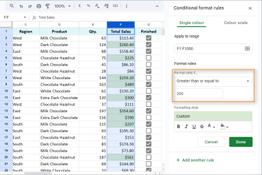 Complete guide to Google Sheets conditional formatting: rules, formulas, use casesApr 09, 2025 am 10:57 AM
Master Google Sheets Conditional Formatting: A Comprehensive Guide This guide provides a complete walkthrough of Google Sheets' conditional formatting, from basic rules to advanced custom formulas. Learn how to highlight key data, save time, and red
 Google Sheets basics: share, move and protect Google SheetsApr 09, 2025 am 10:34 AM
Mastering Google Sheets Collaboration: Sharing, Moving, and Protecting Your Data This "Back to Basics" guide focuses on collaborative spreadsheet management in Google Sheets. Learn how to efficiently share, organize, and protect your data
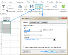 Custom Data Validation in Excel : formulas and rulesApr 09, 2025 am 10:24 AM
This tutorial demonstrates how to create custom data validation rules in Excel. We'll explore several examples, including formulas to restrict input to numbers, text, text starting with specific characters, unique entries, and more. Yesterday's tuto
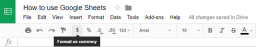 Google Sheets basics: edit, print and download the files in Google SheetsApr 09, 2025 am 10:09 AM
This "Back to Basics" guide delves into essential Google Sheets editing techniques. We'll cover fundamental actions like data deletion and formatting, and then move on to more advanced features such as comments, offline editing, and change
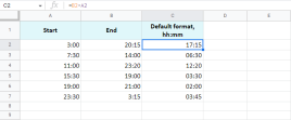 Calculating time in Google SheetsApr 09, 2025 am 09:43 AM
Mastering Google Sheets Time Calculations: A Comprehensive Guide This guide delves into the intricacies of time calculations within Google Sheets, covering time differences, addition/subtraction, summation, and date/time extraction. Calculating Time
 How to use IFERROR in Excel with formula examplesApr 09, 2025 am 09:37 AM
This tutorial demonstrates how Excel's IFERROR function handles errors, replacing them with blanks, alternative values, or custom messages. It covers using IFERROR with VLOOKUP and INDEX MATCH, and compares it to IF ISERROR and IFNA. "Give me a


Hot AI Tools

Undresser.AI Undress
AI-powered app for creating realistic nude photos

AI Clothes Remover
Online AI tool for removing clothes from photos.

Undress AI Tool
Undress images for free

Clothoff.io
AI clothes remover

AI Hentai Generator
Generate AI Hentai for free.

Hot Article
Hot Tools

Notepad++7.3.1
Easy-to-use and free code editor

MantisBT
Mantis is an easy-to-deploy web-based defect tracking tool designed to aid in product defect tracking. It requires PHP, MySQL and a web server. Check out our demo and hosting services.

ZendStudio 13.5.1 Mac
Powerful PHP integrated development environment

SublimeText3 Chinese version
Chinese version, very easy to use

Atom editor mac version download
The most popular open source editor

