


This step-by-step guide will walk you through the process of creating a heat map in Excel with practical examples.
Microsoft Excel is designed to present data in tables. But in some cases, visuals are way easier to comprehend and digest. As you probably know, Excel has a number of inbuilt features to create graphs. Regrettably, a heat map is not on board. Luckily, there is a quick and simple way to create a heat map in Excel with conditional formatting.
What is heat map in Excel?
A heat map (aka heatmap) is a visual interpretation of numeric data where different values are represented by different colors. Typically, warm-to-cool color schemes are employed, so data is represented in the form of hot and cold spots.
Compared to standard analytics reports, heatmaps make it a lot easier to visualize and analyze complex data. They are extensively used by scientists, analysts and marketers for preliminary analysis of data and discovering generic patterns.
Here are a few typical examples:
- Air temperature heat map - is used to visualize air temperature data in a certain region.
- Geographical heat map - displays some numeric data over a geographic area using different shades.
- Risk management heat map - shows different risks and their impacts in a visual and concise way.
In Excel, a heat map is used to depict individual cells in different color-codes based on their values.
For example, from the heatmap below, you can spot the wettest (highlighted in green) and the driest (highlighted in red) regions and decades at a glance:

How to create a heat map in Excel
If you were thinking about coloring each cell depending on its value manually, give up that idea as that would be a needless waste of time. Firstly, it'd take a lot of effort to apply an appropriate color shade according to the value's rank. And secondly, you'd have to redo color-coding every time the values change. Excel conditional formatting effectively overcomes both hurdles.
To make a heat map in Excel, we will be using conditional formatting color scale. Here are the steps to perform:
- Select your dataset. In our case, it's B3:M5.

- On the Home tab, in the Styles group, click Conditional Formatting > Color Scales, and then click the color scale you want. As you hover the mouse over a particular color scale, Excel will show you the live preview directly in your data set.
For this example, we've chosen Red - Yellow - Green color scale:
In the result, you will have the high values highlighted in red, middle in yellow, and low in green. The colors will adjust automatically when the cell values change.


Tip. For the conditional formatting rule to apply to new data automatically, you can convert your data range to a fully-functional Excel table.
Make a heatmap with a custom color scale
When applying a preset color scale, it depicts the lowest, middle and highest values in the predefined colors (green, yellow and red in our case). All the remaining values get different shades of the three main colors.
In case you want to highlight all the cells lower/higher than a given number in a certain color irrespective of their values, then instead of using an inbuilt color scale construct your own one. Here's how to do this:
- On the Home tab, in the Styles group, click Conditional Formatting > Color Scales > More Rules.
- In the New Formatting Rule dialog box, do the following:
- Pick 3-Color scale from the Format Style drop down list.
- For Minimum and/or Maximum value, choose Number in the Type drop down, and enter the desired values in the corresponding boxes.
- For Midpoint, you can set either Number or Percentile (normally, 50%).
- Assign a color to each of the three values.
For this example, we've configured the following settings:
In this custom heatmap, all the temperatures below 45 °F are highlighted in the same shade of green and all the temperatures above 70 °F in the same shade of red:


Create a heat map in Excel without numbers
The heat map you create in Excel is based on the actual cell values and deleting them would destroy the heat map. To hide the cell values without removing them from the sheet, use custom number formatting. Here are the detailed steps:
- Select the heat map.
- Press Ctrl 1 to open the Format Cells dialog.
- On the Number tab, under Category, select Custom.
- In the Type box, type 3 semicolons (;;;).
- Click OK to apply the custom number format.

That's it! Now, your Excel heat map displays only the color-codes without numbers:

Excel heat map with square cells
Another improvement you can make to your heatmap is perfectly square cells. Below is the fastest way to do this without any scripts or VBA codes:
-
Align column headers vertically. To prevent column headers from getting cut off, change their alignment to vertical. This can be done with the help of the Orientation button on the Home tab, in the Alignment group:
For more information, please see How to align text in Excel.
-
Set column width. Select all the columns and drag any column header's edge to make it wider or narrower. As you do this, a tooltip will appear showing an exact pixel count - remember this number.
-
Set row height. Select all the rows and drag any row header's edge to the same pixel value as columns (26 pixels in our case).
Done! All the cells of your hat map are now square shaped:


How to make a heat map in Excel PivotTable
Essentially, creating a heatmap in a pivot table is the same as in a normal data range - by using a conditional formatting color scale. However, there is a caveat: when new data is added to the source table, the conditional formatting will not apply automatically to that data.
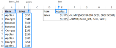
For example, we've added Lui's sales to the source table, refreshed the PivotTable, and see that Lui's numbers are still outside the heat map:

How to make PivotTable heat map dynamic
To force an Excel pivot table heat map to automatically include new entries, here are the steps to perform:
- Select any cell in your current heat map.
- On the Home tab, in the Styles group, click Conditional Formatting > Manage Rules…
- In the Conditional Formatting Rules Manager, select the rule and click on the Edit Rule button.
- In the Edit Formatting Rule dialog box, under Apply Rule To, select the third option. In our case, it reads: All cells showing "Sum of Sales" values for "Reseller" and "Product".
- Click OK twice to close both dialog windows.

Now, your heat map is dynamic and will update automatically as you add new information in the back end. Just remember to refresh your PivotTable :)

How to create a dynamic heat map in Excel with checkbox
If you don't want a heat map to be there all the time, you can hide and show it according to your needs. To create a dynamic heat map with a checkbox, these are the steps to follow:
- Insert a checkbox. Next to your dataset, insert a checkbox (Form control). For this, click the Developer tab > Insert > Form Controls > Checkbox. Here are the detailed steps to add a checkbox in Excel.
-
Link the checkbox to a cell. To link a checkbox to a certain cell, right click the checkbox, click Format Control, switch to the Control tab, enter a cell address into the Cell link box, and click OK.
In our case, the checkbox is linked to cell O2. When the checkbox is selected, the linked cell displays TRUE, otherwise - FALSE.
-
Set up conditional formatting. Select the dataset, click Conditional Formatting > Color Scales > More Rules, and configure a custom color scale in this way:
- In the Format Style drop-down list, select 3-Color Scale.
- Under Minimum, Midpoint and Maximum, select Formula from the Type drop-down list.
- In the Value boxes, enter the following formulas:
For Minimum:
=IF($O$2=TRUE, MIN($B$3:$M$5), FALSE)For Midpoint:
=IF($O$2=TRUE, AVERAGE($B$3:$M$5), FALSE)For Maximum:
=IF($O$2=TRUE, MAX($B$3:$M$5), FALSE)These formulas use the MIN, AVERAGE and MAX functions to work out the lowest, middle and highest values in the dataset (B3:M5) when the linked cell (O2) is TRUE, i.e. when the checkbox is selected.
- In the Color drop-down boxes, choose the desired colors.
- Click the OK button.
Now, the heat map appears only when the checkbox is selected and is hidden the rest of the time.


Tip. To remove the TRUE / FALSE value from view, you can link the checkbox to some cell in an empty column, and then hide that column.
How to make a dynamic heat map in Excel without numbers
To hide numbers in a dynamic heat map, you need to create one more conditional formatting rule that applies a custom number format. Here's how:
- Create a dynamic heat map as explained in the above example.
- Select your data set.
- On the Home tab, in the Styles group, click New Rule > Use a formula to determine which cells to format.
- In the Format values where this formula is true box, enter this formula:
=IF($O$2=TRUE, TRUE, FALSE)Where O2 is your linked cell. The formula says to apply the rule only when the checkbox is checked (O2 is TRUE).
- Click the Format… button.
- In the Format Cells dialog box, switch to the Number tab, select Custom in the Category list, type 3 semicolons (;;;) in the Type box, and click OK.
- Click OK to close the New Formatting Rule dialog box.


From now on, selecting the check box will display the heat map and hide numbers:

To switch between two different heatmap types (with and without numbers), you can insert three radio buttons. And then, configure 3 separate conditional formatting rules: 1 rule for the heat map with numbers, and 2 rules for the heat map without numbers. Or you can create a common color scale rule for both types by using the OR function (as done in our sample worksheet below).
In the result, you will get this nice dynamic heat map:

To better understand how this works, you are welcome to download our sample sheet. Hopefully, this will help you create your own amazing Excel heat map template.
I thank you for reading and hope to see you on our blog next week!
Practice workbook for download
Heat map in Excel - examples (.xlsx file)
The above is the detailed content of How to create a heat map in Excel: static and dynamic. For more information, please follow other related articles on the PHP Chinese website!

 MEDIAN formula in Excel - practical examplesApr 11, 2025 pm 12:08 PM
This tutorial explains how to calculate the median of numerical data in Excel using the MEDIAN function. The median, a key measure of central tendency, identifies the middle value in a dataset, offering a more robust representation of central tenden
 Google Spreadsheet COUNTIF function with formula examplesApr 11, 2025 pm 12:03 PM
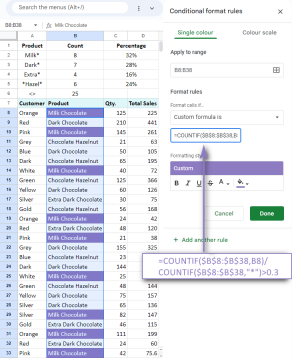
Master Google Sheets COUNTIF: A Comprehensive Guide This guide explores the versatile COUNTIF function in Google Sheets, demonstrating its applications beyond simple cell counting. We'll cover various scenarios, from exact and partial matches to han
 Excel shared workbook: How to share Excel file for multiple usersApr 11, 2025 am 11:58 AM
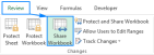
This tutorial provides a comprehensive guide to sharing Excel workbooks, covering various methods, access control, and conflict resolution. Modern Excel versions (2010, 2013, 2016, and later) simplify collaborative editing, eliminating the need to m
 How to convert Excel to JPG - save .xls or .xlsx as image fileApr 11, 2025 am 11:31 AM
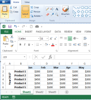
This tutorial explores various methods for converting .xls files to .jpg images, encompassing both built-in Windows tools and free online converters. Need to create a presentation, share spreadsheet data securely, or design a document? Converting yo
 Excel names and named ranges: how to define and use in formulasApr 11, 2025 am 11:13 AM
This tutorial clarifies the function of Excel names and demonstrates how to define names for cells, ranges, constants, or formulas. It also covers editing, filtering, and deleting defined names. Excel names, while incredibly useful, are often overlo
 Standard deviation Excel: functions and formula examplesApr 11, 2025 am 11:01 AM
This tutorial clarifies the distinction between standard deviation and standard error of the mean, guiding you on the optimal Excel functions for standard deviation calculations. In descriptive statistics, the mean and standard deviation are intrinsi
 Square root in Excel: SQRT function and other waysApr 11, 2025 am 10:34 AM
This Excel tutorial demonstrates how to calculate square roots and nth roots. Finding the square root is a common mathematical operation, and Excel offers several methods. Methods for Calculating Square Roots in Excel: Using the SQRT Function: The
 Google Sheets basics: Learn how to work with Google SpreadsheetsApr 11, 2025 am 10:23 AM
Unlock the Power of Google Sheets: A Beginner's Guide This tutorial introduces the fundamentals of Google Sheets, a powerful and versatile alternative to MS Excel. Learn how to effortlessly manage spreadsheets, leverage key features, and collaborate


Hot AI Tools

Undresser.AI Undress
AI-powered app for creating realistic nude photos

AI Clothes Remover
Online AI tool for removing clothes from photos.

Undress AI Tool
Undress images for free

Clothoff.io
AI clothes remover

Video Face Swap
Swap faces in any video effortlessly with our completely free AI face swap tool!

Hot Article
Hot Tools

PhpStorm Mac version
The latest (2018.2.1) professional PHP integrated development tool

SublimeText3 English version
Recommended: Win version, supports code prompts!

mPDF
mPDF is a PHP library that can generate PDF files from UTF-8 encoded HTML. The original author, Ian Back, wrote mPDF to output PDF files "on the fly" from his website and handle different languages. It is slower than original scripts like HTML2FPDF and produces larger files when using Unicode fonts, but supports CSS styles etc. and has a lot of enhancements. Supports almost all languages, including RTL (Arabic and Hebrew) and CJK (Chinese, Japanese and Korean). Supports nested block-level elements (such as P, DIV),

MinGW - Minimalist GNU for Windows
This project is in the process of being migrated to osdn.net/projects/mingw, you can continue to follow us there. MinGW: A native Windows port of the GNU Compiler Collection (GCC), freely distributable import libraries and header files for building native Windows applications; includes extensions to the MSVC runtime to support C99 functionality. All MinGW software can run on 64-bit Windows platforms.

Dreamweaver CS6
Visual web development tools

