


Meet the new Excel TAKE function that can get a specified number of rows or columns from a range or array in a trice.
When working with large arrays of data, you may sometimes need to extract a smaller part for closer examination. With the new dynamic array function introduced in Excel 365, it will be a walk in the park for you. Just specify how many rows and columns you want to take and hit the Enter key :)
TAKE function in Excel
The Excel TAKE function extracts the specified number of contiguous rows and/or columns from the array or range.
The syntax is as follows:
TAKE(array, rows, [columns])Where:
Array (required) - the source array or range.
Rows (optional) - the number of rows to return. A positive value takes rows from the start of the array and a negative value from the end of the array. If omitted, columns must be set.
Columns (optional) - the number of columns to return. A positive integer takes columns from the start of the array and a negative integer from the end of the array. If omitted, rows must be defined.
Here's how the TAKE function looks like:

Tips:
- To return non-adjacent rows from a range, use the CHOOSEROWS function.
- To pull non-adjacent columns, utilize the CHOOSECOLS function.
- To get part of the array by removing a given number of rows or columns, leverage the DROP function.
TAKE function availability
The TAKE function is only supported in Excel for Microsoft 365 (Windows and Mac) and Excel for the web.
In earlier Excel versions, you can use an OFFSET formula as an alternative solution.
How to use TAKE function in Excel
To align expectations and reality when using the TAKE function in your worksheets, take notice of the following things:
- The array argument can be a range of cells or an array of values returned by another formula.
- The rows and columns arguments can be positive or negative integers. Positive numbers take a subset of data from the start of the array; negative numbers - from the end.
- The rows and columns arguments are optional, but at least one of them should be set in a formula. The omitted one defaults to the total number of rows or columns in the array.
- If the rows or columns value is greater than there are rows or columns in the source array, all rows / columns are returned.
- TAKE is a dynamic array function. You enter the formula in only one cell and it automatically spills into as many neighboring cells as needed.
Excel TAKE formula examples
Now that you have a general understanding of how the TAKE function works, let's look at some practical examples to illustrate its real value.
Extract rows from a range or array
To return a given number of contiguous rows from the start of a 2D array or range, supply a positive number for the rows argument.
For example, to take the first 4 rows from the range A3:C14, the formula is:
=TAKE(A3:C14, 4)
The formula lands in cell E3 and spills into four rows and as many columns as there are in the source range.

Take columns from an array or range
To get a certain number of contiguous columns from the start of a 2D array or range, provide a positive number for the columns argument.
For example, to pull the first 2 columns from the range A3:C14, the formula is:
=TAKE(A3:C14, ,2)
The formula goes to cell E3 and spills into two columns and as many rows as there are in the supplied range.

Extract a certain number of rows and columns
To retrieve a given number of rows and columns from the beginning of an array, you provide positive numbers for both the rows and columns arguments.
For example, to take the first 4 rows and 2 columns from our dataset, the formula is:
=TAKE(A3:C14, 4, 2)
Entered in E3, the formula fills four rows (as set in the 2nd argument) and two columns (as defined in the 3rd argument).

Get last N rows
To pull a certain number of rows from the end of an array, provide a negative number for the rows argument. For example:
To take the last row, use -1:
=TAKE(A3:C14, -1)
To get the last 3 rows, supply -3:
=TAKE(A3:C14, -3)
In the screenshot below, you can observe the results.

Return last N columns
To extract some columns from the end of an array or range, use a negative number for the columns argument. For example:
To get the last column, set the 3rd argument to -1:
=TAKE(A3:C14, , -1)
To pull the last 2 columns, set the 3rd argument to -2:
=TAKE(A3:C14, , -2)
And here are the results:

Tip. To take rows and columns from the end of an array, provide negative numbers for both the rows and columns arguments.
How to take rows / columns from multiple ranges
In situation when you want to extract some columns or rows from several non-contiguous ranges, it takes two steps to accomplish the task:
- Combine multiple ranges into one vertically or horizontally using the VSTACK or HSTACK function.
- Return the desired number of columns or rows from the combined array.
Depending on the structure of your worksheet, apply one of the following solutions.
Stack ranges vertically and take rows or columns
Let's say you have 3 separate ranges like shown in the image below. To append each subsequent range to the bottom of the previous one, the formula is:
=VSTACK(A4:C6, A10:C14, A18:C21)
Nest it in the array argument of TAKE, specify how many rows to return, and you will get the result you are looking for:
=TAKE(VSTACK(A4:C6, A10:C14, A18:C21), 4)
To return columns, type the appropriate number in the 3rd argument:
=TAKE(VSTACK(A4:C6, A10:C14, A18:C21), ,2)
The output will look something like this:

Stack ranges horizontally and take rows or columns
In case the data in the source ranges is arranged horizontally in rows, use the HSTACK function to combine them into a single array. For example:
=HSTACK(B3:D5, G3:H5, K3:L5)
And then, you place the above formula inside the TAKE function and set the rows or columns argument, or both, according to your needs.
For example, to get the first 2 rows from the stacked array, the formula is:
=TAKE(HSTACK(B3:D5, G3:H5, K3:L5), 2)
And this formula will bring the last 5 columns:
=TAKE(HSTACK(B3:D5, G3:H5, K3:L5), ,5)

TAKE function alternative for Excel 2010 - 365
In Excel 2019 and earlier versions where the TAKE function is not supported, you can use OFFSET as an alternative. Though the OFFSET formula is not as intuitive and straightforward, it does provide a working solution. And here's how you set it up:
- For the 1st argument, supply the original range of values.
- The 2nd and 3rd arguments or both set to zero or omitted, assuming you are extracting a subset from the beginning of the array. Optionally, you can specify how may rows and columns to offset from the upper-left cell of the array.
- In the 4th argument, indicate the number of rows to return.
- In the 5th argument, define the number of columns to return.
Summing up, the generic formula takes this form:
OFFSET(array, , , rows, columns)For instance, to extract 6 rows and 2 columns from the start of the range A3:C14, the formula goes as follows:
=OFFSET(A3:C14, , , 6, 2)
In all versions except Excel 365 and 2021 that handle arrays natively, this only works as a traditional CSE array formula. There are two ways to enter it:
- Select the range of cells the same size as the expected output (6 rows and 2 columns in our case) and press F2 to enter Edit mode. Type the formula and press Ctrl Shift Enter to enter it in all the selected cells at once.
- Enter the formula in any empty cell (E3 in this example) and press Ctrl Shift Enter to complete it. After that, drag the formula down and to the right across as many rows and columns as needed.
The result will look similar to this:

Note. Please be aware that OFFSET is a volatile function, and it may slow down your worksheet if used in many cells.
Excel TAKE function not working
In case a TAKE formula does not work in your Excel or results in an error, it's most likely to be one of the below reasons.
TAKE is not supported in your version of Excel
TAKE is a new function and it has limited availability. If your version is other than Excel 365, try the alternative OFFSET formula.
Empty array
If either the rows or columns argument is set to 0, a #CALC! error is returned indicating an empty array.
Insufficient number of blank cells to fill with the results
In case there are not enough empty cells for the formula to spill the results into, a #SPILL error occurs. To fix it, just clear the neighboring cells below or/and to the right. For more details, see How to resolve #SPILL! error in Excel.
That's how to use the TAKE function in Excel to extract rows or columns from a range of cells. I thank you for reading and hope to see you on our blog next week!
Practice workbook for download
Excel TAKE formula - examples (.xlsx file)
The above is the detailed content of Excel TAKE function to extract rows or columns from array. For more information, please follow other related articles on the PHP Chinese website!

 MEDIAN formula in Excel - practical examplesApr 11, 2025 pm 12:08 PM
This tutorial explains how to calculate the median of numerical data in Excel using the MEDIAN function. The median, a key measure of central tendency, identifies the middle value in a dataset, offering a more robust representation of central tenden
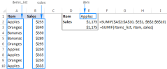
 Google Spreadsheet COUNTIF function with formula examplesApr 11, 2025 pm 12:03 PM
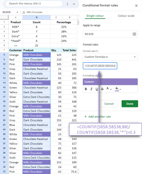
Master Google Sheets COUNTIF: A Comprehensive Guide This guide explores the versatile COUNTIF function in Google Sheets, demonstrating its applications beyond simple cell counting. We'll cover various scenarios, from exact and partial matches to han
 Excel shared workbook: How to share Excel file for multiple usersApr 11, 2025 am 11:58 AM
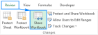
This tutorial provides a comprehensive guide to sharing Excel workbooks, covering various methods, access control, and conflict resolution. Modern Excel versions (2010, 2013, 2016, and later) simplify collaborative editing, eliminating the need to m
 How to convert Excel to JPG - save .xls or .xlsx as image fileApr 11, 2025 am 11:31 AM
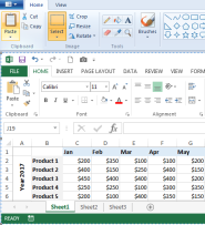
This tutorial explores various methods for converting .xls files to .jpg images, encompassing both built-in Windows tools and free online converters. Need to create a presentation, share spreadsheet data securely, or design a document? Converting yo
 Excel names and named ranges: how to define and use in formulasApr 11, 2025 am 11:13 AM
This tutorial clarifies the function of Excel names and demonstrates how to define names for cells, ranges, constants, or formulas. It also covers editing, filtering, and deleting defined names. Excel names, while incredibly useful, are often overlo
 Standard deviation Excel: functions and formula examplesApr 11, 2025 am 11:01 AM
This tutorial clarifies the distinction between standard deviation and standard error of the mean, guiding you on the optimal Excel functions for standard deviation calculations. In descriptive statistics, the mean and standard deviation are intrinsi
 Square root in Excel: SQRT function and other waysApr 11, 2025 am 10:34 AM
This Excel tutorial demonstrates how to calculate square roots and nth roots. Finding the square root is a common mathematical operation, and Excel offers several methods. Methods for Calculating Square Roots in Excel: Using the SQRT Function: The
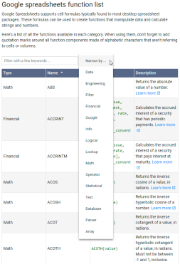 Google Sheets basics: Learn how to work with Google SpreadsheetsApr 11, 2025 am 10:23 AM
Unlock the Power of Google Sheets: A Beginner's Guide This tutorial introduces the fundamentals of Google Sheets, a powerful and versatile alternative to MS Excel. Learn how to effortlessly manage spreadsheets, leverage key features, and collaborate


Hot AI Tools

Undresser.AI Undress
AI-powered app for creating realistic nude photos

AI Clothes Remover
Online AI tool for removing clothes from photos.

Undress AI Tool
Undress images for free

Clothoff.io
AI clothes remover

Video Face Swap
Swap faces in any video effortlessly with our completely free AI face swap tool!

Hot Article
Hot Tools

Dreamweaver CS6
Visual web development tools

PhpStorm Mac version
The latest (2018.2.1) professional PHP integrated development tool

SublimeText3 Chinese version
Chinese version, very easy to use

Notepad++7.3.1
Easy-to-use and free code editor

SublimeText3 Mac version
God-level code editing software (SublimeText3)

