


The fastest way to transform a column or row of values into a two-dimensional array is using the WRAPCOLS or WRAPROWS function.
Since the earliest days of Excel, it has been very good at calculating and analyzing numbers. But manipulating arrays has traditionally been a challenge. The introduction of dynamic arrays made the usage of array formulas a lot easier. And now, Microsoft is releasing a set of new dynamic array functions to manipulate and re-shape arrays. This tutorial will teach you how to use two such functions, WRAPCOLS and WRAPROWS, to transform a column or row into a 2D array in no time.

Excel WRAPCOLS function
The WRAPCOLS function in Excel transforms a row or column of values into a two-dimensional array based on the specified number of values per row.
The syntax has the following arguments:
WRAPCOLS(vector, wrap_count, [pad_with])Where:
- vector (required) - the source one-dimensional array or range.
- wrap_count (required) - the max number of values per column.
- pad_with (optional) - the value to pad with the last column if there are insufficient items to fill it. If omitted, the missing values will be padded with #N/A (default).
For example, to change the range B5:B24 to a 2-dimensional array with 5 values per column, the formula is:
=WRAPROWS(B5:B24, 5)
You enter the formula in any single cell and it automatically spills into as many cells as needed. In the WRAPCOLS output, the values are arranged vertically, from top to bottom, based on the wrap_count value. After the count has been reached, a new column is started.

Excel WRAPROWS function
The WRAPROWS function in Excel converts a row or column of values into a two-dimensional array based on the number of values per row that you specify.
The syntax is as follows:
WRAPROWS(vector, wrap_count, [pad_with])Where:
- vector (required) - the source one-dimensional array or range.
- wrap_count (required) - the max number of values per row.
- pad_with (optional) - the value to pad with the last row if there are insufficient items to fill it. The default is #N/A.
For example, to transform the range B5:B24 into a 2D array having 5 values in each row, the formula is:
=WRAPROWS(B5:B24, 5)
You enter the formula in the upper-left cell of the spill range, and it populates all other cells automatically. The WRAPROWS function arranges the values horizontally, from left to right, based on the wrap_count value. After reaching the count, it starts a new row.

WRAPCOLS and WRAPROWS availability
Both functions are only available in Excel for Microsoft 365 (Windows and Mac) and Excel for the web.
In earlier versions, you can use traditional more complex formulas to perform column-to-array and row-to-array transformations. Further on in this tutorial, we will discuss the alternative solutions in detail.
Tip. To do a reverse operation, i.e. change a 2D array to a single column or row, use the TOCOL or TOROW function, respectively.
How to convert column / row to range in Excel - examples
Now that you've got a grasp of the basic usage, let's take a closer look at a few more specific cases.
Set the maximum number of values per column or row
Depending on the structure of your original data, you may find it suitable to be re-arranged into columns (WRAPCOLS) or rows (WRAPROWS). Whichever function you use, it is the wrap_count argument that determines the max number of values in each column/row.
For example, to transform the range B4:B23 into a 2D array, so that each column has a maximum of 10 values, use this formula:
=WRAPCOLS(B4:B23, 10)
To rearrange the same range by row, so that each row has a maximum of 4 values, the formula is:
=WRAPROWS(B4:B23, 4)
The image below shows how this looks like:

Pad missing values in the resulting array
In case there are insufficient values to fill all the columns/rows of the resulting range, WRAPROWS and WRAPCOLS will return #N/A errors to keep the structure of the 2D array.
To change the default behavior, you can provide a custom value for the optional pad_with argument.
For example, to transform the range B4:B21 into a 2D array with maximum 5 values wide, and pad the last row with dashes if there are not enough data to fill it, use this formula:
=WRAPROWS(B4:B21, 5, "-")
To replace the missing values with zero-length strings (blanks), the formula is:
=WRAPROWS(B4:B21, 5, "")
Please compare the results with the default behavior (formula in D5) where pad_with is omitted:

Merge multiple rows into 2D range
To combine a few separate rows into a single 2D array, you first stack the rows horizontally using the HSTACK function, and then wrap the values using WRAPROWS or WRAPCOLS.
For example, to merge the values from 3 rows (B5:J5, B7:G7 and B9:F9) and wrap into columns, each containing 10 values, the formula is:
=WRAPCOLS(HSTACK(B5:J5, B7:G7, B9:F9), 10)
To combine values from multiple rows into a 2D range where each row contains 5 values, the formula takes this form:
=WRAPROWS(HSTACK(B5:J5, B7:G7, B9:F9), 5)

Combine multiple columns into 2D array
To merge several columns into a 2D range, first you stack them vertically using the VSTACK function, and then wrap the values into rows (WRAPROWS) or columns (WRAPCOLS).
For instance, to combine the values from 3 columns (B5:J5, B7:G7 and B9:F9) into a 2D range where each column contains 10 values, the formula is:
=WRAPCOLS(HSTACK(B5:J5, B7:G7, B9:F9), 10)
To combine the same columns into a 2D range where each row contains 5 values, use this formula:
=WRAPROWS(HSTACK(B5:J5, B7:G7, B9:F9), 5)

Wrap and sort the array
In situation when the source range has values in random order while you wish the output to be sorted, proceed in this way:
- Sort the initial array the way you want using the SORT function.
- Supply the sorted array to WRAPCOLS or WRAPROWS.
For example, to wrap the range B4:B23 into rows, 4 values in each, and sort the resulting range from A to Z, construct a formula like this:
=WRAPROWS(SORT(B4:B23), 4)
To wrap the same range into columns, 10 values in each, and sort the output alphabetically, the formula is:
=WRAPCOLS(SORT(B4:B23), 10)
The results look as follows:

Tip. To arrange the values in the resulting array in descending order, set the third argument (sort_order) of the SORT function to -1.
WRAPCOLS alternative for Excel 365 - 2010
In older Excel versions where the WRAPCOLS function is not supported, you can build your own formula to wrap the values from a one-dimensional array into columns. This can be done by using 5 different functions together.
WRAPCOLS alternative to convert a row into 2D range:
IFERROR(IF(ROW(A1)>n, "", INDEX(row_range, , ROW(A1) (COLUMN(A1)-1)*n)), "")WRAPCOLS alternative to convert a column into 2D range:
IFERROR(IF(ROW(A1)>n, "", INDEX(column_range, ROW(A1) (COLUMN(A1)-1)*n)), "")Where n is the maximum number of values per column.
In the image below, we use the following formula to turn a one-row range (D4:J4) into a three-row array.
=IFERROR(IF(ROW(A1)>3, "", INDEX($D$4:$J$4, , ROW(A1) (COLUMN(A1)-1)*3)), "")
And this formula changes a one-column range (B4:B20) into a five-row array:
=IFERROR(IF(ROW(A1)>5, "", INDEX($B$4:$B$20, ROW(A1) (COLUMN(A1)-1)*5)), "")
The above solutions emulate the analogous WRAPCOLS formulas and produce the same results:
=WRAPCOLS(D4:J4, 3, "")
and
=WRAPCOLS(B4:B20, 5, "")
Please keep in mind that unlike the dynamic array WRAPCOLS function, the traditional formulas follow the one-formula-one-cell approach. So, our first formula is entered in D8 and copied 3 rows down and 3 columns to the right. The second formula is entered in D14 and copied 5 rows down and 4 columns to the right.

How these formulas work
At the heart of both formulas, we use the INDEX function that returns a value from the supplied array based on a row and column number:
INDEX(array, row_num, [column_num])As we are dealing with one-row array, we can omit the row_num argument, so it defaults to 1. The trick is to have col_num calculated automatically for each cell where the formula is copied. And here's how we do this:
ROW(A1) (COLUMN(A1)-1)*3)
The ROW function returns the row number of the A1 reference, which is 1.
The COLUMN function returns the column number of the A1 reference, which is also 1. Subtracting 1 turns it into zero. And multiplying 0 by 3 gives 0.
Then, you add up 1 returned by ROW and 0 returned by COLUMN and get 1 as a result.
This way, the INDEX formula in the upper-left cell of the destination range (D8) undergoes this transformation:
INDEX($D$4:$J$4, ,ROW(A1) (COLUMN(A1)-1)*3))
changes to
INDEX($D$4:$J$4, ,1)
and returns the value from the 1st column of the specified array, which is "Apples" in D4.
When the formula is copied to cell D9, the relative cell references change based on a relative position of rows and columns while the absolute range reference remains unchanged:
INDEX($D$4:$J$4,, ROW(A2) (COLUMN(A2)-1)*3))
turns into:
INDEX($D$4:$J$4,, 2 (1-1)*3))
becomes:
INDEX($D$4:$J$4,, 2))
and returns the value from the 2nd column of the specified array, which is "Apricots" in E4.
The IF function checks the row number and if it's greater than the number of rows you specified (3 in our case) returns an empty string (""), otherwise the result of the INDEX function:
IF(ROW(A1)>3, "", INDEX(…))
Finally, the IFERROR function fixes a #REF! error that occurs when the formula is copied to more cells than really needed.
The second formula that converts a column into 2D range works with the same logic. The difference is that you use the ROW COLUMN combination to figure out the row_num argument for INDEX. The col_num parameter is not needed in this case since there is just one column in the source array.
WRAPROWS alternative for Excel 365 - 2010
To wrap the values from a one-dimensional array into rows in Excel 2019 and earlier, you can use the following alternatives to the WRAPROWS function.
Transform a row into 2D range:
IFERROR(IF(COLUMN(A1)>n, "", INDEX(row_range, , COLUMN(A1) (ROW(A1)-1)*n)), "")Change a column to 2D range:
IFERROR(IF(COLUMN(A1)>n, "", INDEX(column_range, COLUMN(A1) (ROW(A1)-1)*n)), "")Where n is the maximum number of values per row.
In our sample data set, we use the following formula to convert a one-row range (D4:J4) into a three-column range. The formula lands in cell D8, and then is copied across 3 columns and 3 rows.
=IFERROR(IF(COLUMN(A1)>3, "", INDEX($D$4:$J$4, , COLUMN(A1) (ROW(A1)-1)*3)), "")
To reshape a 1-column range (B4:B20) into a 5-column range, enter the below formula in D14 and drag it across 5 columns and 4 rows.
=IFERROR(IF(COLUMN(A1)>5, "", INDEX($B$4:$B$20, COLUMN(A1) (ROW(A1)-1)*5)), "")
In Excel 365, the same results can be achieved with the equivalent WRAPCOLS formulas:
=WRAPROWS(D4:J4, 3, "")
and
=WRAPROWS(B4:B20, 5, "")

How these formulas work
Essentially, these formulas work like in the previous example. The difference is in how you determine the row_num and col_num coordinates for the INDEX function:
INDEX($D$4:$J$4,, COLUMN(A1) (ROW(A1)-1)*3))
To get the column number for the upper left cell in the destination range (D8), you use this expression:
COLUMN(A1) (ROW(A1)-1)*3)
that changes to:
1 (1-1)*3
and gives 1.
As a result, the below formula returns the value from the first column of the specified array, which is "Apples":
INDEX($D$4:$J$4,, 1)
So far, the result is the same as in the previous example. But let's see what happens in other cells…
In cell D9, the relative cell references change as follows:
INDEX($D$4:$J$4,, COLUMN(A2) (ROW(A2)-1)*3))
So, the formula transforms into:
INDEX($D$4:$J$4,, 1 (2-1)*3))
becomes:
INDEX($D$4:$J$4,, 4))
and returns the value from the 4th column of the specified array, which is "Cherries" in G4.
The IF function checks the column number and if it's greater than the number of columns you specified, returns an empty string (""), otherwise the result of the INDEX function:
IF(COLUMN(A1)>3, "", INDEX(…))
As a finishing touch, IFERROR prevents #REF! errors from appearing in "extra" cells if you copy the formula to more cells than actually needed.
WRAPCOLS or WRAPROWS function not working
If the "wrap" functions are not available in your Excel or result in an error, it's most likely to be one of below reasons.
#NAME? error
In Excel 365, a #NAME? error may occur because you misspelled the function's name. In other versions, it indicates that the functions are not supported. As a workaround, you can use WRAPCOLS alternative or WRAPROWS alternative.
#VALUE! error
A #VALUE error occurs if the vector argument is not a one-dimensional array.
#NUM! error
A #NUM error occurs if the wrap_count value is 0 or negative number.
#SPILL! error
Most often, a #SPILL error indicates that there are not enough blank cells to spill the results into. Clear the neighboring cells, and it will be gone. If the error persists, check out what #SPILL means in Excel and how to fix it.
That's how to use the WRAPCOLS and WRAPROWS functions to convert a one-dimensional range into a two-dimensional array in Excel. I thank you for reading and hope to see you on our blog next week!
Practice workbook for download
WRAPCOLS and WRAPROWS functions - examples (.xlsx file)
The above is the detailed content of Convert column / row to array in Excel: WRAPCOLS & WRAPROWS functions. For more information, please follow other related articles on the PHP Chinese website!

 MEDIAN formula in Excel - practical examplesApr 11, 2025 pm 12:08 PM
This tutorial explains how to calculate the median of numerical data in Excel using the MEDIAN function. The median, a key measure of central tendency, identifies the middle value in a dataset, offering a more robust representation of central tenden
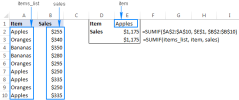
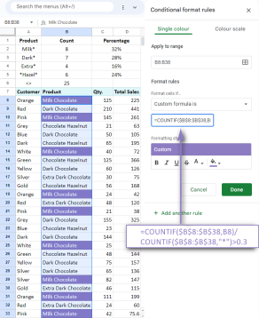 Google Spreadsheet COUNTIF function with formula examplesApr 11, 2025 pm 12:03 PM
Master Google Sheets COUNTIF: A Comprehensive Guide This guide explores the versatile COUNTIF function in Google Sheets, demonstrating its applications beyond simple cell counting. We'll cover various scenarios, from exact and partial matches to han
 Excel shared workbook: How to share Excel file for multiple usersApr 11, 2025 am 11:58 AM
This tutorial provides a comprehensive guide to sharing Excel workbooks, covering various methods, access control, and conflict resolution. Modern Excel versions (2010, 2013, 2016, and later) simplify collaborative editing, eliminating the need to m
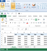 How to convert Excel to JPG - save .xls or .xlsx as image fileApr 11, 2025 am 11:31 AM
This tutorial explores various methods for converting .xls files to .jpg images, encompassing both built-in Windows tools and free online converters. Need to create a presentation, share spreadsheet data securely, or design a document? Converting yo
 Excel names and named ranges: how to define and use in formulasApr 11, 2025 am 11:13 AM
This tutorial clarifies the function of Excel names and demonstrates how to define names for cells, ranges, constants, or formulas. It also covers editing, filtering, and deleting defined names. Excel names, while incredibly useful, are often overlo
 Standard deviation Excel: functions and formula examplesApr 11, 2025 am 11:01 AM
This tutorial clarifies the distinction between standard deviation and standard error of the mean, guiding you on the optimal Excel functions for standard deviation calculations. In descriptive statistics, the mean and standard deviation are intrinsi
 Square root in Excel: SQRT function and other waysApr 11, 2025 am 10:34 AM
This Excel tutorial demonstrates how to calculate square roots and nth roots. Finding the square root is a common mathematical operation, and Excel offers several methods. Methods for Calculating Square Roots in Excel: Using the SQRT Function: The
 Google Sheets basics: Learn how to work with Google SpreadsheetsApr 11, 2025 am 10:23 AM
Unlock the Power of Google Sheets: A Beginner's Guide This tutorial introduces the fundamentals of Google Sheets, a powerful and versatile alternative to MS Excel. Learn how to effortlessly manage spreadsheets, leverage key features, and collaborate


Hot AI Tools

Undresser.AI Undress
AI-powered app for creating realistic nude photos

AI Clothes Remover
Online AI tool for removing clothes from photos.

Undress AI Tool
Undress images for free

Clothoff.io
AI clothes remover

Video Face Swap
Swap faces in any video effortlessly with our completely free AI face swap tool!

Hot Article
Hot Tools

SublimeText3 Linux new version
SublimeText3 Linux latest version

ZendStudio 13.5.1 Mac
Powerful PHP integrated development environment

DVWA
Damn Vulnerable Web App (DVWA) is a PHP/MySQL web application that is very vulnerable. Its main goals are to be an aid for security professionals to test their skills and tools in a legal environment, to help web developers better understand the process of securing web applications, and to help teachers/students teach/learn in a classroom environment Web application security. The goal of DVWA is to practice some of the most common web vulnerabilities through a simple and straightforward interface, with varying degrees of difficulty. Please note that this software

EditPlus Chinese cracked version
Small size, syntax highlighting, does not support code prompt function

SAP NetWeaver Server Adapter for Eclipse
Integrate Eclipse with SAP NetWeaver application server.

