Mastering Image Segmentation: How Traditional Techniques Still Shine in the Digital Age

Introduction

Image segmentation, one of the most basic procedures in computer vision, allows a system to decompose and analyze various regions within an image. Whether you're dealing with object recognition, medical imaging, or autonomous driving, segmentation is what breaks images down into meaningful parts.

Although deep learning models continue to be increasingly popular in this task, traditional techniques in digital image processing still are powerful and practical. The approaches being reviewed in this post include thresholding, edge detection, region-based, and clustering by implementing a well-recognized dataset for the analysis of cell images, the MIVIA HEp-2 Image Dataset.

MIVIA HEp-2 Image Dataset

The MIVIA HEp-2 Image Dataset is a set of pictures of the cells used to analyze the pattern of antinuclear antibodies (ANA) through HEp-2 cells. It consists of 2D pictures taken through fluorescence microscopy. This makes it very suitable for segmentation tasks, most importantly those concerned with medical image analysis, where cellular region detection is most important.

Now, let's move on to the segmentation techniques used to process these images, comparing their performance based on the F1 scores.

---

1. Thresholding Segmentation

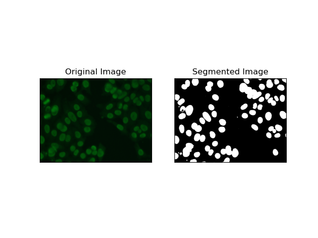
Thresholding is the process whereby grayscale images get converted into binary images based on pixel intensities. In the MIVIA HEp-2 dataset, this process is useful in cell extraction from the background. It is simple and effective to a relatively large level, especially with Otsu's method, as it self-computes the optimum threshold.

Otsu's Method is an automatic thresholding method, where it tries to find the best threshold value to yield the minimal intra-class variance, thereby separating the two classes: foreground (cells) and background. The method examines the image histogram and computes the perfect threshold, where the sum of the pixel intensity variances in each class is minimized.

# Thresholding Segmentation
def thresholding(img):
    # Convert image to grayscale
    gray = cv.cvtColor(img, cv.COLOR_BGR2GRAY)

    # Apply Otsu's thresholding
    _, thresh = cv.threshold(gray, 0, 255, cv.THRESH_BINARY + cv.THRESH_OTSU)

    return thresh

---

2. Edge Detection Segmentation

Edge detection pertains to identifying boundaries of objects or regions, such as cell edges in the MIVIA HEp-2 dataset. Of the many available methods for detecting abrupt intensity changes, the Canny Edge Detector is the best and hence most appropriate method to be used for detecting cellular boundaries.

Canny Edge Detector is a multi-stage algorithm that can detect the edges by detecting areas of strong gradients of intensity. The process embodies smoothing with a Gaussian filter, calculation of intensity gradients, application of non-maximum suppression to eliminate spurious responses, and a final double thresholding operation for the retention of only salient edges.

# Edge Detection Segmentation
def edge_detection(img):
    # Convert image to grayscale
    gray = cv.cvtColor(img, cv.COLOR_BGR2GRAY)

    # Apply Gaussian blur
    gray = cv.GaussianBlur(gray, (3, 3), 0)

    # Calculate lower and upper thresholds for Canny edge detection
    sigma = 0.33
    v = np.median(gray)
    lower = int(max(0, (1.0 - sigma) * v))
    upper = int(min(255, (1.0 + sigma) * v))

    # Apply Canny edge detection
    edges = cv.Canny(gray, lower, upper)

    # Dilate the edges to fill gaps
    kernel = np.ones((5, 5), np.uint8)
    dilated_edges = cv.dilate(edges, kernel, iterations=2)

    # Clean the edges using morphological opening
    cleaned_edges = cv.morphologyEx(dilated_edges, cv.MORPH_OPEN, kernel, iterations=1)

    # Find connected components and filter out small components
    num_labels, labels, stats, _ = cv.connectedComponentsWithStats(
        cleaned_edges, connectivity=8
    )
    min_size = 500
    filtered_mask = np.zeros_like(cleaned_edges)
    for i in range(1, num_labels):
        if stats[i, cv.CC_STAT_AREA] >= min_size:
            filtered_mask[labels == i] = 255

    # Find contours of the filtered mask
    contours, _ = cv.findContours(
        filtered_mask, cv.RETR_EXTERNAL, cv.CHAIN_APPROX_SIMPLE
    )

    # Create a filled mask using the contours
    filled_mask = np.zeros_like(gray)
    cv.drawContours(filled_mask, contours, -1, (255), thickness=cv.FILLED)

    # Perform morphological closing to fill holes
    final_filled_image = cv.morphologyEx(
        filled_mask, cv.MORPH_CLOSE, kernel, iterations=2
    )

    # Dilate the final filled image to smooth the edges
    final_filled_image = cv.dilate(final_filled_image, kernel, iterations=1)

    return final_filled_image

---

3. Region-Based Segmentation

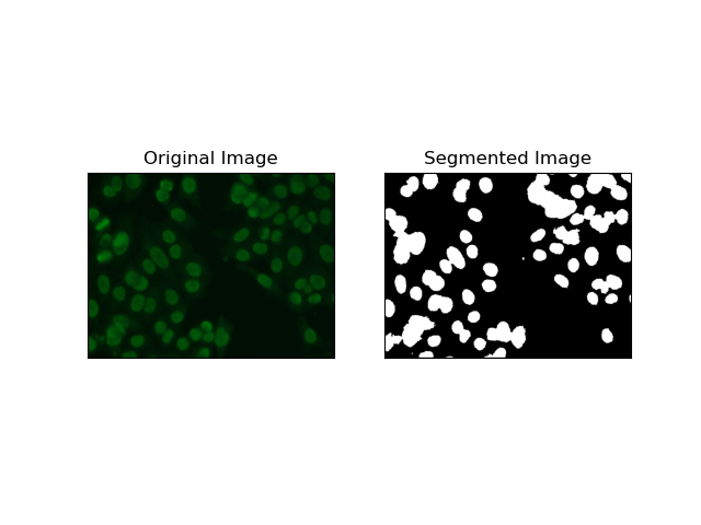
Region-based segmentation groups similar pixels together into regions, dependent on certain criteria such as intensity or color. The Watershed segmentation technique can be used to help in segmenting HEp-2 cell images to be able to detect those regions that represent cells; it considers pixel intensities as a topographic surface and outlines distinguishing regions.

Watershed segmentation treats the intensities of pixels as a topographical surface. The algorithm identifies "basins" in which it identifies local minima and then gradually floods these basins to enlarge distinct regions. This technique is quite useful when one wants to separate touching objects, like in the case of cells within microscopic images, but it can be sensitive to noise. The process can be guided by markers and over-segmentation can often be reduced.

# Region-Based Segmentation
def region_based(img):
    # Convert image to grayscale
    gray = cv.cvtColor(img, cv.COLOR_BGR2GRAY)

    # Apply Otsu's thresholding
    _, thresh = cv.threshold(gray, 0, 255, cv.THRESH_BINARY_INV + cv.THRESH_OTSU)

    # Apply morphological opening to remove noise
    kernel = np.ones((3, 3), np.uint8)
    opening = cv.morphologyEx(thresh, cv.MORPH_OPEN, kernel, iterations=2)

    # Dilate the opening to get the background
    sure_bg = cv.dilate(opening, kernel, iterations=3)

    # Calculate the distance transform
    dist_transform = cv.distanceTransform(opening, cv.DIST_L2, 5)

    # Threshold the distance transform to get the foreground
    _, sure_fg = cv.threshold(dist_transform, 0.2 * dist_transform.max(), 255, 0)
    sure_fg = np.uint8(sure_fg)

    # Find the unknown region
    unknown = cv.subtract(sure_bg, sure_fg)

    # Label the markers for watershed algorithm
    _, markers = cv.connectedComponents(sure_fg)
    markers = markers + 1
    markers[unknown == 255] = 0

    # Apply watershed algorithm
    markers = cv.watershed(img, markers)

    # Create a mask for the segmented region
    mask = np.zeros_like(gray, dtype=np.uint8)
    mask[markers == 1] = 255

    return mask

---

4. Clustering-Based Segmentation

Clustering techniques such as K-Means tend to group the pixels into similar clusters, which works fine when wanting to segment cells in multi-colored or complex environments, as seen in HEp-2 cell images. Fundamentally, this could represent different classes, such as a cellular region versus a background.

K-means is an unsupervised learning algorithm for clustering images based on the pixel similarity of color or intensity. The algorithm randomly selects K centroids, assigns each pixel to the nearest centroid, and updates the centroid iteratively until it converges. It is particularly effective in segmenting an image that has multiple regions of interest that are very different from one another.

# Clustering Segmentation
def clustering(img):
    # Convert image to grayscale
    gray = cv.cvtColor(img, cv.COLOR_BGR2GRAY)

    # Reshape the image
    Z = gray.reshape((-1, 3))
    Z = np.float32(Z)

    # Define the criteria for k-means clustering
    criteria = (cv.TERM_CRITERIA_EPS + cv.TERM_CRITERIA_MAX_ITER, 10, 1.0)

    # Set the number of clusters
    K = 2

    # Perform k-means clustering
    _, label, center = cv.kmeans(Z, K, None, criteria, 10, cv.KMEANS_RANDOM_CENTERS)

    # Convert the center values to uint8
    center = np.uint8(center)

    # Reshape the result
    res = center[label.flatten()]
    res = res.reshape((gray.shape))

    # Apply thresholding to the result
    _, res = cv.threshold(res, 0, 255, cv.THRESH_BINARY + cv.THRESH_OTSU)

    return res

---

Evaluating the Techniques Using F1 Scores

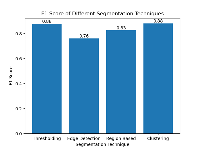
The F1 score is a measure that combines precision and recall together to compare the predicted segmentation image with the ground truth image. It is the harmonic mean of precision and recall, which is useful in cases of high data imbalance, such as in medical imaging datasets.

We calculated the F1 score for each segmentation method by flattening both the ground truth and the segmented image and calculating the weighted F1 score.

def calculate_f1_score(ground_image, segmented_image):
    ground_image = ground_image.flatten()
    segmented_image = segmented_image.flatten()
    return f1_score(ground_image, segmented_image, average="weighted")

We then visualized the F1 scores of different methods using a simple bar chart:

---

Conclusion

Although many recent approaches for image segmentation are emerging, traditional segmentation techniques such as thresholding, edge detection, region-based methods, and clustering can be very useful when applied to datasets such as the MIVIA HEp-2 image dataset.

Each method has its strength:

• Thresholding is good for simple binary segmentation.
• Edge Detection is an ideal technique for the detection of boundaries.
• Region-based segmentation is very useful in separating connected components from their neighbors.
• Clustering methods are well-suited for multi-region segmentation tasks.

By evaluating these methods using F1 scores, we understand the trade-offs each of these models has. These methods may not be as sophisticated as what is developed in the newest models of deep learning, but they are still fast, interpretable, and serviceable in a broad range of applications.

---

Thanks for reading! I hope this exploration of traditional image segmentation techniques inspires your next project. Feel free to share your thoughts and experiences in the comments below!

The above is the detailed content of Mastering Image Segmentation: How Traditional Techniques Still Shine in the Digital Age. For more information, please follow other related articles on the PHP Chinese website!