

 Technology peripheralsAIOverview of path planning: based on sampling, search, and optimization, all done!
1 Overview of decision control and motion planning
Currently decision control methods can be divided into three categories: sequential planning, behavior-aware planning, and end-to-end planning .

- sequential planning: the most traditional method, perception, decision-making and control The levels of each part are relatively clear;
- behavior-aware planning: Compared with the first type, the highlight is the introduction of human-machine co-driving, vehicle-road collaboration, and vehicle risk estimation of the external dynamic environment;
- End-to-end planning: DL and DRL technology uses a large amount of data training to obtain the relationship from sensory information such as images to vehicle control inputs such as steering wheel angle. It is one of the most popular methods nowadays.
This article will introduce sequential planning, follow the entire decision-making control sequence and describe the perception control process of autonomous vehicles. Finally, it will briefly summarize the issues to be solved mentioned above. question.

Control architecture for automated vehicles
2 Overview of path planning
The process of sequential planning is briefly summarized asPath Planning->Decision-making process->Vehicle Control, the path planning described in this article belongs to the first and third steps.

https://www.php.cn/link/aa7d66ed4b1c618962d406535c4d282a
On the issue of motion trajectory generation of unmanned vehicles , there are direct trajectory generation method and path-speed decomposition method. Compared with the first method, path-speed is less difficult, so it is more commonly used.
2.1 Types of path planning
Path planning can be divided into four major categories: sampling-based algorithms represented by PRM and RRT, Algorithms based on search represented by A* and D*, trajectory generation algorithms based on interpolationfitting represented by β-splines, and MPC represented by Optimal control algorithm for local path planning. This section will explain them one by one in the order mentioned above:

A Review of Motion Planning Techniques for Automated Vehicles
2.2 Advantages and Disadvantages of Path Planning Algorithms

3 Path planning method
3.1 Sampling-based algorithm
3.1.1 Basic algorithm PRM and RRT

(1) PRM
PRM algorithm (Probabilistic Road Map) . PRM mainly consists of two steps, one is the learning stage, and the other is the query stage.
The first step, the learning stage: uniformly and randomly sample n points in the safe area in the state space, and delete the points where the samples fall on the obstacles, and then connect the adjacent points and perform collision detection. , eliminate the connections that are not collision-free, and finally obtain a connected graph.
The second step, the query stage: for a given pair of initial and target states, use the sampling nodes and continuity constructed in the previous step, and use the graph search method (Dijkstra or A*) to find a feasible path.
After completing the PRM construction, it can be used to solve motion planning problems in different initial and target states, but this feature is unnecessary for unmanned vehicle motion planning. In addition, PRM requires precise connections between states, which is very difficult for motion planning problems with complex differential constraints.
(2) RRT
RRT (Rapidly-exploring Random Tree) algorithm. RRT actually represents a series of algorithms based on the idea of randomly growing trees. It is currently the most widely used algorithm with the most optimized variants in the field of robotics.

① Tree initialization: Initialize the node set and edge set of the tree. The node set only contains the initial state and the edge set is empty;
② Tree growth: Randomly sample the state space. When the sampling point falls in the safe area of the state space, select the node closest to the sampling point in the current tree and extend it to the sampling point; if the generated trajectory does not If it collides with an obstacle, the trajectory is added to the edge set of the tree, and the end point of the trajectory is added to the node set of the tree
③ Repeat step ② until it is expanded to the target state set. Compared with PRM, there is no In terms of graphs, RRT constructs a tree structure with the initial state as the root node and the target state as the leaf node. For different initial and target states, different trees need to be constructed.
RRT does not require precise connections between states and is more suitable for solving motion dynamics problems such as unmanned vehicle motion planning.
3.1.2 Problems and Solutions of Sampling Method
Solution efficiency and whether it is the optimal solution. The reason why PRM and RRT have probabilistic completeness is that they will traverse almost all positions in the configuration space.
(1) Solving efficiency
In terms of improving solving efficiency, the core idea of optimizing RRT is to guide the tree to the open area, that is, try to stay away from obstacles and avoid repeated checks of nodes at obstacles to improve efficiency. Main solution:
① Uniform sampling
The standard RRT algorithm samples the state spaceuniformly and randomly, and the nodes in the current tree obtain The probability of expansion is proportional to the area of its Voronoi region, so the tree will grow towards the empty area of the state space, evenly filling the free area of the state space.
The RRT-connect algorithm simultaneously constructs two trees starting from the initial state and the target state. When the two trees grow together then a feasible solution is found. Go-biaing inserts the target state at a certain proportion in the random sampling sequence, guiding the tree to expand toward the target state, speeding up the solution speed, and improving the solution quality.
Heuristic RRT uses a heuristic function to increase the probability of sampling nodes with low expansion costs and calculate the cost of each node in the tree. However, in complex environments, the definition of the cost function is difficult. In order to solve this problem For one problem, the f-biased sampling method first discretizes the state space into a grid, and then uses the Dijkstra algorithm to calculate the cost on each grid. The cost value of the points in the area of the grid is equal to this value, thereby constructing a heuristic formula function.
② Optimize distance measurement
Distance is used to measure the cost of the path between two configurations, assists in generating a heuristic cost function, and guides the direction of the tree. However, distance calculation is difficult when obstacles are considered. The definition of distance in motion planning adopts a definition similar to Euclidean distance. RG-RRT (rechability guided RRT) can eliminate the impact of inaccurate distance on RRT exploration ability. It needs to calculate the reachable set of nodes in the tree. When the distance from the sampling point to the node is greater than the reachable set of the node, distance, the node may be selected for expansion.
③ Reduce the number of collision checks
One of the efficiency bottlenecks of the collision check sampling method, the usual approach is to discretize the path at equal distances, Then perform a collision check on the configuration at each point. resolution complete RRT obtains the probability of expansion by reducing nodes close to obstacles. It discretizes the input space and only uses it once for a certain node input; if the trajectory corresponding to a certain input collides with an obstacle , then a penalty value is added to the node. The higher the penalty value, the smaller the probability of the node being expanded. Dynamic domain RRT and adaptive dynamic domain RRT limit the sampling area to the local space where the current tree is located to prevent nodes close to obstacles from repeated expansion failures and improve algorithm efficiency.
④ Improve real-time performance
Anytime RRT first quickly builds an RRT, obtains a feasible solution and records its cost, and then continues sampling, but it will only help reduce the feasibility The node with the solution cost is inserted into the tree, thereby gradually obtaining a better feasible solution. Replanning decomposes the entire planning task into a number of equal-time sub-task sequences, and plans the next task while executing the current task.
(2) There are mainly the following methods to solve the optimality problem:
RGG algorithm (random geometric graph): According to the random geometric graph theory, the standard PRM and RRT is an improved PRM, RRG and RRT algorithm with asymptotic optimal properties. It randomly samples n points in the state space and connects the points whose distance is less than r(n) to form RGG. . RRT* Algorithm: Introduce the "reconnection" step based on RRG to check whether the newly inserted node as the parent node of its adjacent point will reduce the cost of its adjacent points. If it does, remove the adjacent points. Click the original parent-child relationship and use the current insertion point as its parent node. This is the RRT* algorithm.
LBT-RRT algorithm: A large number of node connections and local adjustments make PRM and RRT very inefficient. The LBT-RRT algorithm combines the RRG and RRT* algorithms to obtain higher efficiency on the premise of obtaining asymptotic optimality.
3.2 Search-based algorithm
The basic idea is to discretize the state spacein a certain way into a graph, and then use each A heuristic search algorithmsearchesfeasible solutionsor evenoptimal solutions, this category algorithm is relatively mature.

The basis of the search-based algorithm is the state lattice. The state lattice is the discretization of the state space, consisting of the state node and the movement starting from the node to the adjacent node. Composed of primitives, one state node can be transformed to another state node through its motion primitives. The state lattice converts the original continuous state space into a search graph. The motion planning problem becomes searching for a series of motion primitives that transform the initial state to the target state in the graph. After constructing the state lattice, you can use graph search algorithm to search for the optimal trajectory.
3.2.1 Construction of basic algorithms Dijkstra and A*
Dijkstra algorithm traverses the entire configuration space, finds the distance between each two grids, and finally selects The shortest path from the starting point to the target point has a very low efficiency due to its breadth-first nature. On the basis of this algorithm, adding a heuristic function, that is, the distance from the searched node to the target node, and searching again based on this can avoid The inefficiency caused by global search is the A* algorithm, as shown in the figure below, the red is the search area.

Figure 6: Comparison of the effects of A* and Dijkstra algorithms
3.2.2 Problems and suggestions of search methods
Same as sampling-based algorithms, this type of algorithm also needs to be optimized for efficiency and optimality.
In terms of improving efficiency, A* itself is a static planning algorithm. An extension of the A* algorithm is weighted A*, which further guides the search direction to the target node by increasing the weight of the heuristic function, improving the search speed. It is fast, but it is easy to fall into local minima and cannot guarantee the global optimal solution.
For moving vehicles, using A*’s derivative algorithm D (dynamic A) can greatly improve efficiency. Also based on dynamic programming is LPA. This algorithm can handle the situation where the cost of the motion primitives of the state grid is time-varying. When the environment changes, a new optimal plan can be planned by re-searching a smaller number of nodes. path. Developed on the basis of LPA , D*-Lite can achieve the same results as D*, but with higher efficiency.
When searching for optimal solutions, ARA* is an Anytime search algorithm developed on the basis of Weighted A*. It calls the Weighted A* algorithm multiple times and narrows down the heuristics with each call. The weight of the formula function allows the algorithm to quickly find a feasible solution. By introducing the set INCONS, each cycle can continue to use the information of the previous cycle to optimize the path and gradually approach the optimal solution.
On the issue of balancing algorithm efficiency and optimality, Sandin aine et al. proposed the MHA* algorithm, which introduced multiple heuristic functions to ensure that one of the heuristic functions can find the optimal solution when used alone. , so that by coordinating the path costs generated by different heuristic functions, the efficiency and optimality of the algorithm can be taken into account. DMHA generates appropriate heuristic functions online and in real time based on MHA, thereby avoiding the local minimum problem.
3.3 Algorithm based on interpolation fitting

The algorithm based on interpolation fitting can be defined as: according to a known The series is used to describe the point set of the road map. By using data interpolation and curve fitting, the path that the smart car will travel can be created. Provide better continuity and higher derivability. The specific method is as follows:
Dubins curve and Reeds and Sheep (RS) curve are the shortest paths connecting any two points in the configuration space, corresponding to the situations without reversing and with reversing respectively. They are all composed of arcs of maximum curvature and straight lines. There is a curvature discontinuity at the connection between the arc and the straight line. When an actual vehicle travels on such a curve, it must stop and adjust the steering wheel at the discontinuity of curvature to continue driving.
Polynomial interpolation curve is the most commonly used method. It can set polynomial coefficients by meeting the requirements of nodes and obtain better continuous differentiability. Fourth-order polynomials It is often used in longitudinal constraint control, fifth-order polynomials are often used in lateral constraint control, and third-order polynomials are also used in overtaking trajectories.
Spline curve has a closed expression and can easily ensure curvature continuity. β-spline curves can achieve curvature continuity, and cubic Bezier curves can ensure the continuity and boundedness of curvature, and the amount of calculation is relatively small. The η^3 curve [43] is a seven-degree spline curve, which has very good properties: continuity of curvature and continuity of curvature derivatives, which is very meaningful for high-speed vehicles.
3.4 Algorithms based on optimal control
Algorithms based on optimal control are classified into path planning, mainly because the MPC can perform local path planning For obstacle avoidance, in addition, the main function of MPC is trajectory tracking. In addition to the necessary dynamics and kinematic constraints, the issues it considers should also consider comfort, uncertainty of sensory information, and workshop in the future. communication uncertainty, and the driver can also be included in the control loop during local trajectory planning. The above-mentioned uncertainty issues and incorporating the driver into the control loop will be discussed in Section 4. Regarding the study of MPC, we mainly start from two aspects: optimization theory and engineering practice. For the former, I recommend Convex Optimization Algorithms by Dimitri P. Bertsekas and Model Predictive Control: Theory, Computation, and Design by James B. Rawlings. In the Chinese field, teacher Liu Haoyang’s optimization book personally feels that it is relatively clear and easy to understand. For the latter, first of all, Teacher Gong Jianwei’s self-driving MPC book is strongly recommended. There were problems with the demo in the old version of the book, but they were all solved in the new version.
There are many types of prediction models used by MPC: such as convolutional neural network, fuzzy control, state space, etc. Among them, the most commonly used is the state space method. MPC can be briefly expressed as: when the necessary dynamics, kinematics, etc. constraints are met, the optimal solution of the model is solved through numerical means. The optimal solution is the control variable of the state equation, such as the steering wheel angle, etc., and Apply the control quantity to the car model to obtain the required state quantities, such as speed, acceleration, coordinates, etc.
It can be seen from the above description that the key to MPC lies in the establishment and solution of the model. How to equivalently simplify the establishment of the model and improve the efficiency of the solution is the top priority. The vehicle will take different trajectories under different control inputs, and each trajectory corresponds to an objective function value. The unmanned vehicle will use a solving algorithm to find the control quantity corresponding to the minimum objective function value, and apply it to the vehicle. As shown in the figure below:

In order to reduce the difficulty of modeling, artificial potential energy field models are also used for modeling. The basic idea of artificial potential energy fields is similar to electric fields. On the road Obstacles are analogous to charges in an electric field that are of a different polarity than the source of the field. The potential energy at obstacles (dynamic, static) is higher, and the unmanned vehicle will move toward a low potential energy position.
4 Open source project
Recommend an open source project CppRobotics:
- Path Planning
- Dijkstra
- A Star
- RRT
- Dynamic Window Approach
- Model Predictive Trajectory Generator
- Cubic Spline Planner
- State Lattice Planner
- Frenet Frame Trajectory
5 Learning method
The learning context for entry into new fields is: Engineering, Theory and Vision Troika go hand in hand, taking path planning as an example:
5.1 Engineering
refers to understanding each path planning algorithm Content, while understanding the content of each algorithm from breadth, while learning the details of each algorithm from depth. Regarding algorithms in the field of path planning, there is currently no comprehensive tutorial, but Gong Jianwei's NMPC motion planning can be a reference.
5.2 Theory
refers to understanding the mathematical principles that support the operation of these algorithms and the reasons why these algorithms are generated (mathematical perspective).
- Constructing the objective function and constraint conditions while seeking the extreme value to obtain the optimal control quantity (path), which belongs to Optimization theory;
- is solving the optimal problem The common numerical solution methods such as Newton's method and steepest descent method when controlling quantities essentially come from numerically solving algebraic equations and belong to numerical analysis;
- What you see during the solution process The obtained derivative Jacobian matrix, vector norms in judgment conditions, etc. are essentially the solution of one-dimensional numerical calculations to high dimensions, which belongs to matrix theory.
5.3 Vision
refers to understanding the main applications of path planning in scientific research and enterprises, using scientific research documents and results reports, etc.
6 Summary
This article introduces the outline of current path planning and understands the current path planning methods. The content is very complicated, and it is difficult to learn it all in a short period of time without practical application orientation. You can only focus on learning when needed.
The above is the detailed content of Overview of path planning: based on sampling, search, and optimization, all done!. For more information, please follow other related articles on the PHP Chinese website!

 在 CARLA自动驾驶模拟器中添加真实智体行为Apr 08, 2023 pm 02:11 PM
arXiv论文“Insertion of real agents behaviors in CARLA autonomous driving simulator“,22年6月,西班牙。由于需要快速prototyping和广泛测试,仿真在自动驾驶中的作用变得越来越重要。基于物理的模拟具有多种优势和益处,成本合理,同时消除了prototyping、驾驶员和弱势道路使用者(VRU)的风险。然而,主要有两个局限性。首先,众所周知的现实差距是指现实和模拟之间的差异,阻碍模拟自主驾驶体验去实现有效的现实世界
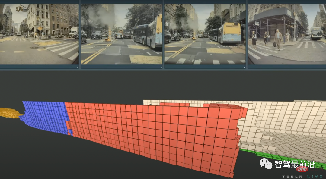 特斯拉自动驾驶算法和模型解读Apr 11, 2023 pm 12:04 PM
特斯拉是一个典型的AI公司,过去一年训练了75000个神经网络,意味着每8分钟就要出一个新的模型,共有281个模型用到了特斯拉的车上。接下来我们分几个方面来解读特斯拉FSD的算法和模型进展。01 感知 Occupancy Network特斯拉今年在感知方面的一个重点技术是Occupancy Network (占据网络)。研究机器人技术的同学肯定对occupancy grid不会陌生,occupancy表示空间中每个3D体素(voxel)是否被占据,可以是0/1二元表示,也可以是[0, 1]之间的
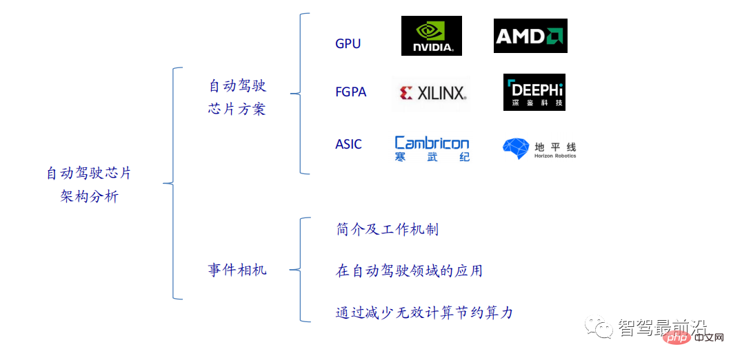 一文通览自动驾驶三大主流芯片架构Apr 12, 2023 pm 12:07 PM
当前主流的AI芯片主要分为三类,GPU、FPGA、ASIC。GPU、FPGA均是前期较为成熟的芯片架构,属于通用型芯片。ASIC属于为AI特定场景定制的芯片。行业内已经确认CPU不适用于AI计算,但是在AI应用领域也是必不可少。 GPU方案GPU与CPU的架构对比CPU遵循的是冯·诺依曼架构,其核心是存储程序/数据、串行顺序执行。因此CPU的架构中需要大量的空间去放置存储单元(Cache)和控制单元(Control),相比之下计算单元(ALU)只占据了很小的一部分,所以CPU在进行大规模并行计算
 自动驾驶汽车激光雷达如何做到与GPS时间同步?Mar 31, 2023 pm 10:40 PM
gPTP定义的五条报文中,Sync和Follow_UP为一组报文,周期发送,主要用来测量时钟偏差。 01 同步方案激光雷达与GPS时间同步主要有三种方案,即PPS+GPRMC、PTP、gPTPPPS+GPRMCGNSS输出两条信息,一条是时间周期为1s的同步脉冲信号PPS,脉冲宽度5ms~100ms;一条是通过标准串口输出GPRMC标准的时间同步报文。同步脉冲前沿时刻与GPRMC报文的发送在同一时刻,误差为ns级别,误差可以忽略。GPRMC是一条包含UTC时间(精确到秒),经纬度定位数据的标准格
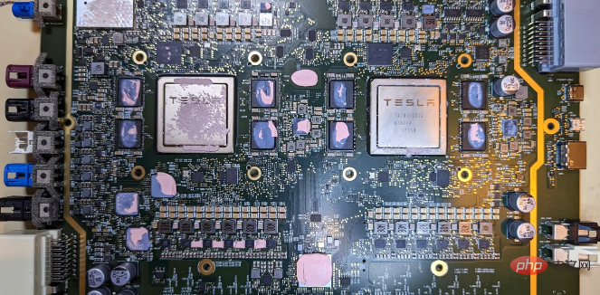 特斯拉自动驾驶硬件 4.0 实物拆解:增加雷达,提供更多摄像头Apr 08, 2023 pm 12:11 PM
2 月 16 日消息,特斯拉的新自动驾驶计算机,即硬件 4.0(HW4)已经泄露,该公司似乎已经在制造一些带有新系统的汽车。我们已经知道,特斯拉准备升级其自动驾驶硬件已有一段时间了。特斯拉此前向联邦通信委员会申请在其车辆上增加一个新的雷达,并称计划在 1 月份开始销售,新的雷达将意味着特斯拉计划更新其 Autopilot 和 FSD 的传感器套件。硬件变化对特斯拉车主来说是一种压力,因为该汽车制造商一直承诺,其自 2016 年以来制造的所有车辆都具备通过软件更新实现自动驾驶所需的所有硬件。事实证
 端到端自动驾驶中轨迹引导的控制预测:一个简单有力的基线方法TCPApr 10, 2023 am 09:01 AM
arXiv论文“Trajectory-guided Control Prediction for End-to-end Autonomous Driving: A Simple yet Strong Baseline“, 2022年6月,上海AI实验室和上海交大。当前的端到端自主驾驶方法要么基于规划轨迹运行控制器,要么直接执行控制预测,这跨越了两个研究领域。鉴于二者之间潜在的互利,本文主动探索两个的结合,称为TCP (Trajectory-guided Control Prediction)。具
 一文聊聊自动驾驶中交通标志识别系统Apr 12, 2023 pm 12:34 PM
什么是交通标志识别系统?汽车安全系统的交通标志识别系统,英文翻译为:Traffic Sign Recognition,简称TSR,是利用前置摄像头结合模式,可以识别常见的交通标志 《 限速、停车、掉头等)。这一功能会提醒驾驶员注意前面的交通标志,以便驾驶员遵守这些标志。TSR 功能降低了驾驶员不遵守停车标志等交通法规的可能,避免了违法左转或者无意的其他交通违法行为,从而提高了安全性。这些系统需要灵活的软件平台来增强探测算法,根据不同地区的交通标志来进行调整。交通标志识别原理交通标志识别又称为TS
 一文聊聊SLAM技术在自动驾驶的应用Apr 09, 2023 pm 01:11 PM
定位在自动驾驶中占据着不可替代的地位,而且未来有着可期的发展。目前自动驾驶中的定位都是依赖RTK配合高精地图,这给自动驾驶的落地增加了不少成本与难度。试想一下人类开车,并非需要知道自己的全局高精定位及周围的详细环境,有一条全局导航路径并配合车辆在该路径上的位置,也就足够了,而这里牵涉到的,便是SLAM领域的关键技术。什么是SLAMSLAM (Simultaneous Localization and Mapping),也称为CML (Concurrent Mapping and Localiza


Hot AI Tools

Undresser.AI Undress
AI-powered app for creating realistic nude photos

AI Clothes Remover
Online AI tool for removing clothes from photos.

Undress AI Tool
Undress images for free

Clothoff.io
AI clothes remover

AI Hentai Generator
Generate AI Hentai for free.

Hot Article
Hot Tools

MinGW - Minimalist GNU for Windows
This project is in the process of being migrated to osdn.net/projects/mingw, you can continue to follow us there. MinGW: A native Windows port of the GNU Compiler Collection (GCC), freely distributable import libraries and header files for building native Windows applications; includes extensions to the MSVC runtime to support C99 functionality. All MinGW software can run on 64-bit Windows platforms.

DVWA
Damn Vulnerable Web App (DVWA) is a PHP/MySQL web application that is very vulnerable. Its main goals are to be an aid for security professionals to test their skills and tools in a legal environment, to help web developers better understand the process of securing web applications, and to help teachers/students teach/learn in a classroom environment Web application security. The goal of DVWA is to practice some of the most common web vulnerabilities through a simple and straightforward interface, with varying degrees of difficulty. Please note that this software

Safe Exam Browser
Safe Exam Browser is a secure browser environment for taking online exams securely. This software turns any computer into a secure workstation. It controls access to any utility and prevents students from using unauthorized resources.

SAP NetWeaver Server Adapter for Eclipse
Integrate Eclipse with SAP NetWeaver application server.

mPDF
mPDF is a PHP library that can generate PDF files from UTF-8 encoded HTML. The original author, Ian Back, wrote mPDF to output PDF files "on the fly" from his website and handle different languages. It is slower than original scripts like HTML2FPDF and produces larger files when using Unicode fonts, but supports CSS styles etc. and has a lot of enhancements. Supports almost all languages, including RTL (Arabic and Hebrew) and CJK (Chinese, Japanese and Korean). Supports nested block-level elements (such as P, DIV),

